Probability and statistics
Inclusion–exclusion, conditional probability, Bayes trees, expectation and variance, the law of large numbers, the central limit theorem, Poisson arrivals, the 3σ rule, Monte Carlo π, random walks and hypothesis tests.
This page lists 12 examples. The code is imported from corpus/examples/math-prob/; the screenshots are end states rendered on real machines.
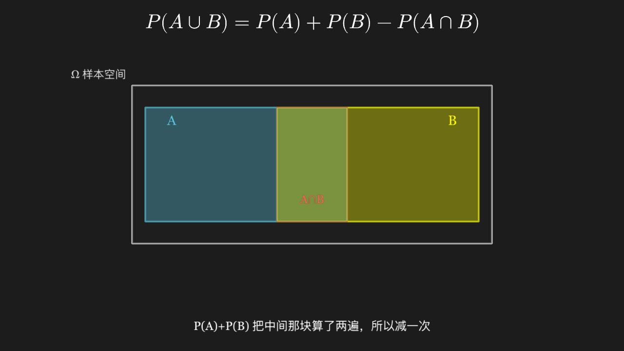
Addition rule (inclusion–exclusion): P(A∪B) = P(A) + P(B) - P(A∩B)
Inside the sample space Ω two translucent rectangular events A and B overlap, the overlap mixing into an intermediate colour; A∩B is lit separately with a red stroked frame and a letter label, then the formula shows it is exactly the part counted twice.
"""概率的加法公式(容斥):P(A∪B) = P(A) + P(B) - P(A∩B)

@expect 样本空间 Ω 里两个半透明矩形事件 A、B 相互交叠,重叠区由两层填色混出中间色;A∩B 用红色描边框单独点亮并标注字母,再回到公式里说明它刚好是被重复计入的那一份。
@note 讲解要点:容斥公式的「减一次交集」不是凑出来的修正项——P(A)+P(B) 把 A∩B 里的概率计了两遍,减掉它才算不重不漏。
"""

from manim import *


class InclusionExclusionScene(Scene):
    def construct(self):
        space = Rectangle(width=8.2, height=3.6, color=GRAY_B).move_to([0, 0.25, 0])
        space.set_fill(GRAY_E, opacity=0.35)

        a_box = Rectangle(width=4.6, height=2.6, color=BLUE).move_to([-1.5, 0.25, 0])
        b_box = Rectangle(width=4.6, height=2.6, color=YELLOW).move_to([1.5, 0.25, 0])
        inter = Rectangle(width=1.6, height=2.6, color=RED).move_to([0, 0.25, 0])
        a_box.set_fill(BLUE, opacity=0.35)
        b_box.set_fill(YELLOW, opacity=0.35)
        inter = Rectangle(width=1.6, height=2.6, color=RED, stroke_width=3).move_to([0, 0.25, 0])

        label_omega = Text("Ω 样本空间", font_size=24, color=GRAY_A).next_to(space, UL, buff=0.14)
        label_a = Text("A", font_size=30, color=BLUE).move_to([-3.2, 1.25, 0])
        label_b = Text("B", font_size=30, color=YELLOW).move_to([3.2, 1.25, 0])
        label_inter = Text("A∩B", font_size=26, color=RED).move_to([0, -0.55, 0])

        formula = MathTex(r"P(A\cup B) = P(A) + P(B) - P(A\cap B)", font_size=44).to_edge(UP, buff=0.3)
        caption = Text(
            "P(A)+P(B) 把中间那块算了两遍,所以减一次",
            font_size=26,
        ).to_edge(DOWN, buff=0.4)

        self.play(Create(space), Write(label_omega), run_time=0.8)
        self.play(Write(formula), run_time=0.8)
        self.play(Create(a_box), Create(b_box), Write(label_a), Write(label_b), run_time=1.0)
        self.play(Create(inter), Write(label_inter), run_time=0.6)
        self.play(Circumscribe(inter, color=WHITE, stroke_width=3), run_time=0.9)
        self.play(Write(caption), run_time=0.7)
        self.wait(0.4)
Conditional probability: renormalizing on a new sample space
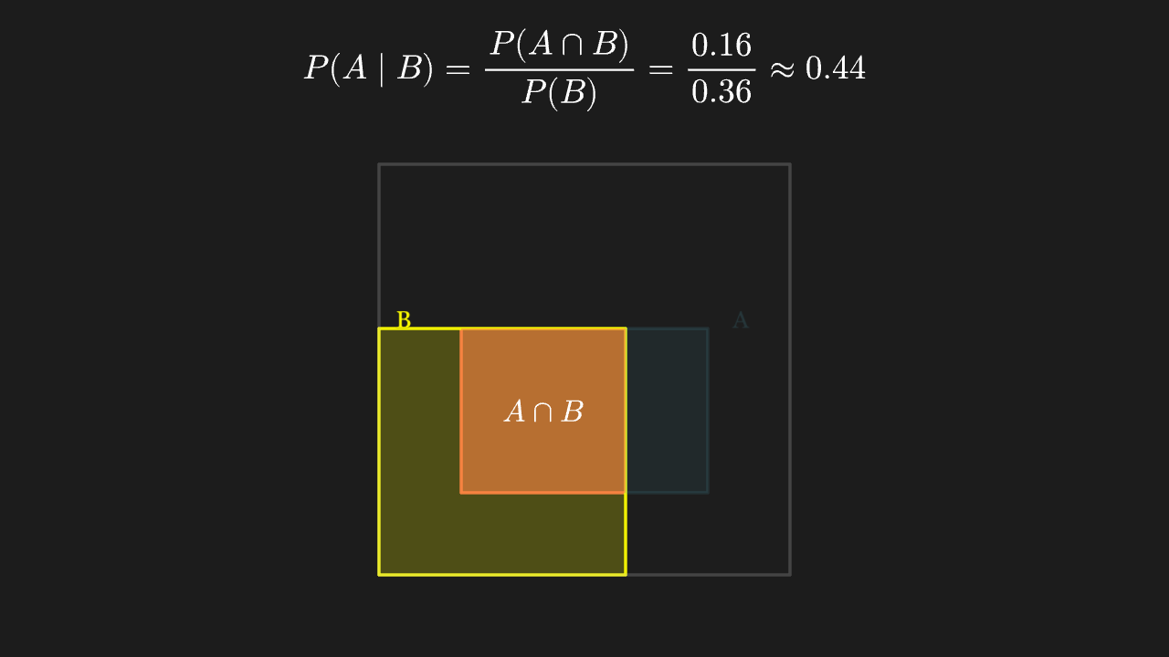
Event A is cut in two by B's boundary; the half inside B is lit first, then everything outside B dims as a whole and only the interior of B is rescaled proportionally.
"""条件概率:换一个样本空间重新归一化

@expect 事件 A 被 B 的边界切成两半,先点亮落在 B 里的那一半;随后 B 之外的部分整体压暗,只剩 B 内部重新按比例摊开。
@note 讲解要点:P(A|B) 的分母从 Ω 换成了 B——不是给 A 打折扣,而是「已知 B 发生」之后把概率全部压回 B 内部重新分配。
"""

from manim import *


class ConditionalProbabilityScene(Scene):
    def construct(self):
        omega = Rectangle(width=5.0, height=5.0, color=GRAY_B).move_to([0, -0.5, 0])
        omega.set_fill(GRAY_E, opacity=0.3)

        b_box = Rectangle(width=3.0, height=3.0, color=YELLOW).move_to([-1.0, -1.5, 0])
        b_box.set_fill(YELLOW, opacity=0.22)

        a_inside = Rectangle(width=2.0, height=2.0, color=RED).move_to([-0.5, -1.0, 0])
        a_outside = Rectangle(width=1.0, height=2.0, color=BLUE).move_to([1.0, -1.0, 0])
        a_inside.set_fill(RED, opacity=0.6)
        a_outside.set_fill(BLUE, opacity=0.6)

        label_a = Text("A", font_size=28, color=BLUE).move_to([1.9, 0.1, 0])
        label_b = Text("B", font_size=28, color=YELLOW).move_to([-2.2, 0.1, 0])
        label_ab = MathTex(r"A\cap B", font_size=36, color=WHITE).move_to([-0.5, -1.0, 0])

        formula = MathTex(
            r"P(A\mid B) = \frac{P(A\cap B)}{P(B)} = \frac{0.16}{0.36} \approx 0.44",
            font_size=40,
        ).to_edge(UP, buff=0.35)

        self.play(Create(omega), run_time=0.6)
        self.play(Write(formula), run_time=0.8)
        self.play(Create(a_outside), Create(a_inside), Write(label_a), run_time=0.8)
        self.play(Create(b_box), Write(label_b), run_time=0.7)
        self.play(Write(label_ab), Indicate(a_inside, color=WHITE, scale_factor=1.05), run_time=0.8)
        self.play(
            a_outside.animate.set_opacity(0.12),
            a_inside.animate.set_opacity(1.0),
            omega.animate.set_opacity(0.25),
            b_box.animate.set_opacity(1.0),
            label_a.animate.set_opacity(0.15),
            run_time=1.0,
        )
        self.wait(0.4)
Bayes' formula: a tree combining prior and likelihood into posterior
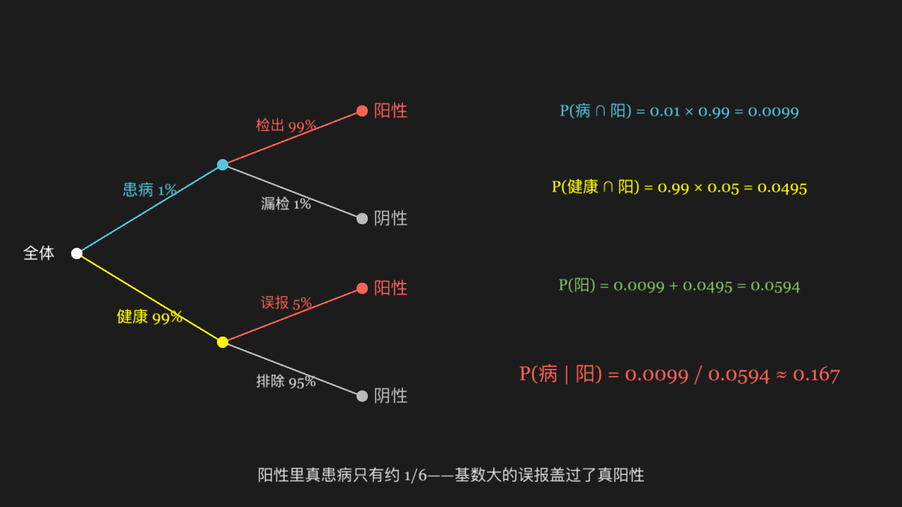
A two-level branching tree on the left lays out the two routes sick 1% × detected 99% and healthy 99% × false alarm 5%; the right lists both joint probabilities — the green total positive probability is the denominator and the red route's share is the posterior.
"""贝叶斯公式:一棵树上把先验和似然合成后验

@expect 左侧两层分叉的树把「患病 1% × 检出 99%」和「健康 99% × 误报 5%」两条路分别铺开;右侧列出两条路的联合概率,绿色那条阳性总概率是分母,红色那条占比就是后验。
@note 讲解要点:阳性结果里真患病只占约 1/6——因为健康人基数大,哪怕误报率只有 5%,误报的绝对数量也远大于真阳性。这就是「基率」被忽略的代价。
"""

from manim import *

ROOT = [-5.9, 0, 0]
LV2_SICK = [-3.6, 1.4, 0]
LV2_WELL = [-3.6, -1.4, 0]
LV3_POS_SICK = [-1.4, 2.25, 0]
LV3_NEG_SICK = [-1.4, 0.55, 0]
LV3_POS_WELL = [-1.4, -0.55, 0]
LV3_NEG_WELL = [-1.4, -2.25, 0]


class BayesTreeScene(Scene):
    def construct(self):
        branch = lambda a, b, c=GRAY_B: Line(a, b, color=c, stroke_width=2.5)

        trunk = VGroup(branch(ROOT, LV2_SICK, BLUE), branch(ROOT, LV2_WELL, YELLOW))
        upper = VGroup(branch(LV2_SICK, LV3_POS_SICK, RED), branch(LV2_SICK, LV3_NEG_SICK))
        lower = VGroup(branch(LV2_WELL, LV3_POS_WELL, RED), branch(LV2_WELL, LV3_NEG_WELL))

        root_dot = Dot(ROOT, radius=0.09, color=WHITE)
        level2_dots = VGroup(
            Dot(LV2_SICK, radius=0.09, color=BLUE),
            Dot(LV2_WELL, radius=0.09, color=YELLOW),
        )
        leaves = VGroup(
            Dot(LV3_POS_SICK, radius=0.09, color=RED),
            Dot(LV3_NEG_SICK, radius=0.09, color=GRAY_B),
            Dot(LV3_POS_WELL, radius=0.09, color=RED),
            Dot(LV3_NEG_WELL, radius=0.09, color=GRAY_B),
        )

        head_labels = VGroup(
            Text("全体", font_size=24).move_to([-6.5, 0, 0]),
            Text("患病 1%", font_size=24, color=BLUE).move_to([-4.75, 1.0, 0]),
            Text("健康 99%", font_size=24, color=YELLOW).move_to([-4.75, -1.0, 0]),
        )
        rate_labels = VGroup(
            Text("检出 99%", font_size=22, color=RED).move_to([-2.6, 2.02, 0]),
            Text("漏检 1%", font_size=22, color=GRAY_A).move_to([-2.6, 0.78, 0]),
            Text("误报 5%", font_size=22, color=RED).move_to([-2.6, -0.78, 0]),
            Text("排除 95%", font_size=22, color=GRAY_A).move_to([-2.6, -2.02, 0]),
        )
        leaf_labels = VGroup(
            Text("阳性", font_size=26, color=RED).move_to([-0.95, 2.25, 0]),
            Text("阴性", font_size=26, color=GRAY_B).move_to([-0.95, 0.55, 0]),
            Text("阳性", font_size=26, color=RED).move_to([-0.95, -0.55, 0]),
            Text("阴性", font_size=26, color=GRAY_B).move_to([-0.95, -2.25, 0]),
        )

        line_sick_pos = Text("P(病 ∩ 阳) = 0.01 × 0.99 = 0.0099", font_size=24, color=BLUE)
        line_sick_pos.move_to([3.6, 2.25, 0])
        line_well_pos = Text("P(健康 ∩ 阳) = 0.99 × 0.05 = 0.0495", font_size=24, color=YELLOW)
        line_well_pos.move_to([3.6, 1.05, 0])
        line_total = Text("P(阳) = 0.0099 + 0.0495 = 0.0594", font_size=24, color=GREEN)
        line_total.move_to([3.6, -0.5, 0])
        posterior = Text("P(病 | 阳) = 0.0099 / 0.0594 ≈ 0.167", font_size=30, color=RED)
        posterior.move_to([3.6, -1.9, 0])

        caption = Text("阳性里真患病只有约 1/6——基数大的误报盖过了真阳性", font_size=24, color=GRAY_A)
        caption.to_edge(DOWN, buff=0.35)

        self.play(Create(trunk), FadeIn(root_dot), run_time=0.8)
        self.play(Write(head_labels), FadeIn(level2_dots), run_time=0.8)
        self.play(Create(upper), Create(lower), FadeIn(leaves), run_time=1.0)
        self.play(Write(rate_labels), run_time=0.9)
        self.play(Write(leaf_labels), run_time=0.8)
        self.play(Write(line_sick_pos), Write(line_well_pos), run_time=0.9)
        self.play(Write(line_total), run_time=0.7)
        self.play(Write(posterior), run_time=0.9)
        self.play(Write(caption), run_time=0.8)
        self.wait(0.4)
Expectation: the centre of mass of a distribution, and this lever's fulcrum
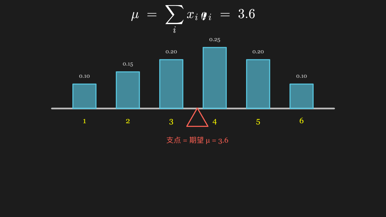
Blocks whose heights are proportional to probabilities stand at six values, and the lever balances exactly at the weighted mean μ=3.6 — not at the arithmetic centre 3.5.
"""期望:概率分布的「重心」,也是这根杠杆的支点

@expect 六个取值位置上立着高度正比于概率的方块,杠杆在正中间找到平衡——支点恰好落在加权平均 μ=3.6 处,而不是算术中心 3.5。
@note 讲解要点:期望就是「按概率加权后的平均位置」。概率大的取值把支点拉向自己,和物理杠杆完全同构——这也是期望才叫「均值」的原因。
"""

from manim import *


class ExpectationBalanceScene(Scene):
    def construct(self):
        faces = [1, 2, 3, 4, 5, 6]
        weights = [0.10, 0.15, 0.20, 0.25, 0.20, 0.10]
        mean = sum(f * w for f, w in zip(faces, weights))

        x_at = lambda face: -4.0 + (face - 1) * 1.6
        beam = Line([-5.2, 0, 0], [5.2, 0, 0], color=GRAY_B, stroke_width=6)

        blocks = VGroup()
        for face, w in zip(faces, weights):
            block = Rectangle(width=0.85, height=w * 9.0, color=BLUE)
            block.set_fill(BLUE, opacity=0.65)
            block.move_to([x_at(face), w * 9.0 / 2, 0])
            blocks.add(block)

        face_labels = VGroup()
        for face in faces:
            face_labels.add(
                Text(str(face), font_size=28, color=YELLOW).move_to([x_at(face), -0.45, 0])
            )

        weight_labels = VGroup()
        for face, w in zip(faces, weights):
            weight_labels.add(
                Text(f"{w:.2f}", font_size=20, color=GRAY_A).move_to([x_at(face), w * 9.0 + 0.3, 0])
            )

        pivot_x = x_at(mean)
        fulcrum = Triangle(color=RED).scale(0.45).move_to([pivot_x, -0.32, 0])
        pivot_label = Text("支点 = 期望 μ = 3.6", font_size=26, color=RED)
        pivot_label.next_to(fulcrum, DOWN, buff=0.35)

        # MathTex 定位用绝对坐标:to_edge 要读包围盒,包围盒由 KaTeX 异步量出,量出前是 NaN(时隐时现)
        formula = MathTex(r"\mu \;=\; \sum_i x_i\, p_i \;=\; 3.6", font_size=48).move_to([0, 3.3, 0])

        self.play(Write(formula), run_time=1.0)
        self.play(Create(beam), run_time=0.5)
        self.play(LaggedStart(*[FadeIn(b) for b in blocks], lag_ratio=0.1), run_time=1.4)
        self.play(Write(face_labels), Write(weight_labels), run_time=0.8)
        self.play(FadeIn(fulcrum), Write(pivot_label), run_time=0.8)
        self.play(Indicate(blocks[3], color=RED, scale_factor=1.06), run_time=0.6)
        self.wait(0.4)
Variance measures spread: same expectation, different scatter
Two data sets share one number line and one mean tick, yet one crowds into a clump while the other spreads wide; two range bars with end ticks mark each spread, and the visual gap corresponds directly to variances 2 and 200.
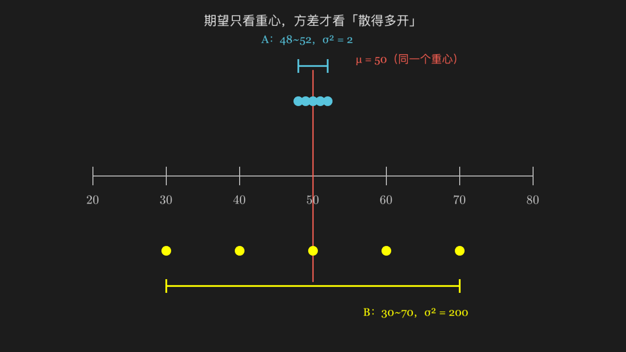
"""方差刻画离散程度:同期望,不同「撒得开」

@expect 上下一共两组数据共享同一条数轴和同一个均值刻度,但一组的点挤成一撮、另一组散得很开;两条两端带短竖线端点标记的横线标出各自的极差,视觉差距直接对应方差 2 与 200。
@note 讲解要点:均值只告诉你「重心在哪」,完全说不出「有多散」——两组数据 μ 都是 50,却是完全不同的两个分布。方差就是把这个「散」量化出来的量。
"""

from manim import *


class VarianceSpreadScene(Scene):
    def construct(self):
        group_a = [48, 49, 50, 51, 52]
        group_b = [30, 40, 50, 60, 70]
        x_of = lambda v: -5.0 + (v - 20) / 6.0

        axis = NumberLine(
            x_range=[20, 80, 10],
            length=10.0,
            include_numbers=True,
            color=GRAY_B,
        )
        mean_line = Line([0, -2.4, 0], [0, 2.4, 0], color=RED, stroke_width=3)

        dots_a = VGroup(*[Dot([x_of(v), 1.7, 0], radius=0.11, color=BLUE) for v in group_a])
        dots_b = VGroup(*[Dot([x_of(v), -1.7, 0], radius=0.11, color=YELLOW) for v in group_b])

        def span_line(x1, x2, y, color):
            bar = Line([x1, y, 0], [x2, y, 0], color=color, stroke_width=4)
            cap_l = Line([x1, y - 0.14, 0], [x1, y + 0.14, 0], color=color, stroke_width=4)
            cap_r = Line([x2, y - 0.14, 0], [x2, y + 0.14, 0], color=color, stroke_width=4)
            return VGroup(bar, cap_l, cap_r)

        span_a = span_line(x_of(48), x_of(52), 2.5, BLUE)
        span_b = span_line(x_of(30), x_of(70), -2.5, YELLOW)

        txt = lambda s, c=WHITE, fs=26: Text(s, font_size=fs, color=c)
        labels = VGroup(
            txt("μ = 50(同一个重心)", RED, 24).next_to(mean_line, UP, buff=0.1).shift(RIGHT * 2.2),
            txt("A:48~52,σ² = 2", BLUE, 24).move_to([x_of(48) + 0.2, 3.1, 0]),
            txt("B:30~70,σ² = 200", YELLOW, 24).move_to([x_of(70) - 1.0, -3.1, 0]),
        )

        title = txt("期望只看重心,方差才看「散得多开」", GRAY_A, 28).to_edge(UP, buff=0.3)

        self.play(Write(title), run_time=0.7)
        self.play(Create(axis), run_time=0.7)
        self.play(FadeIn(dots_a), Create(span_a), Write(labels[1]), run_time=1.0)
        self.play(Create(mean_line), Write(labels[0]), run_time=0.8)
        self.play(FadeIn(dots_b), Create(span_b), Write(labels[2]), run_time=1.0)
        self.wait(0.4)
Law of large numbers: frequency settling onto the true probability
A polyline starts with violent oscillation and narrows towards the dashed line y=0.5 as trials accumulate — convergence holds with probability 1, not monotonically at every step.
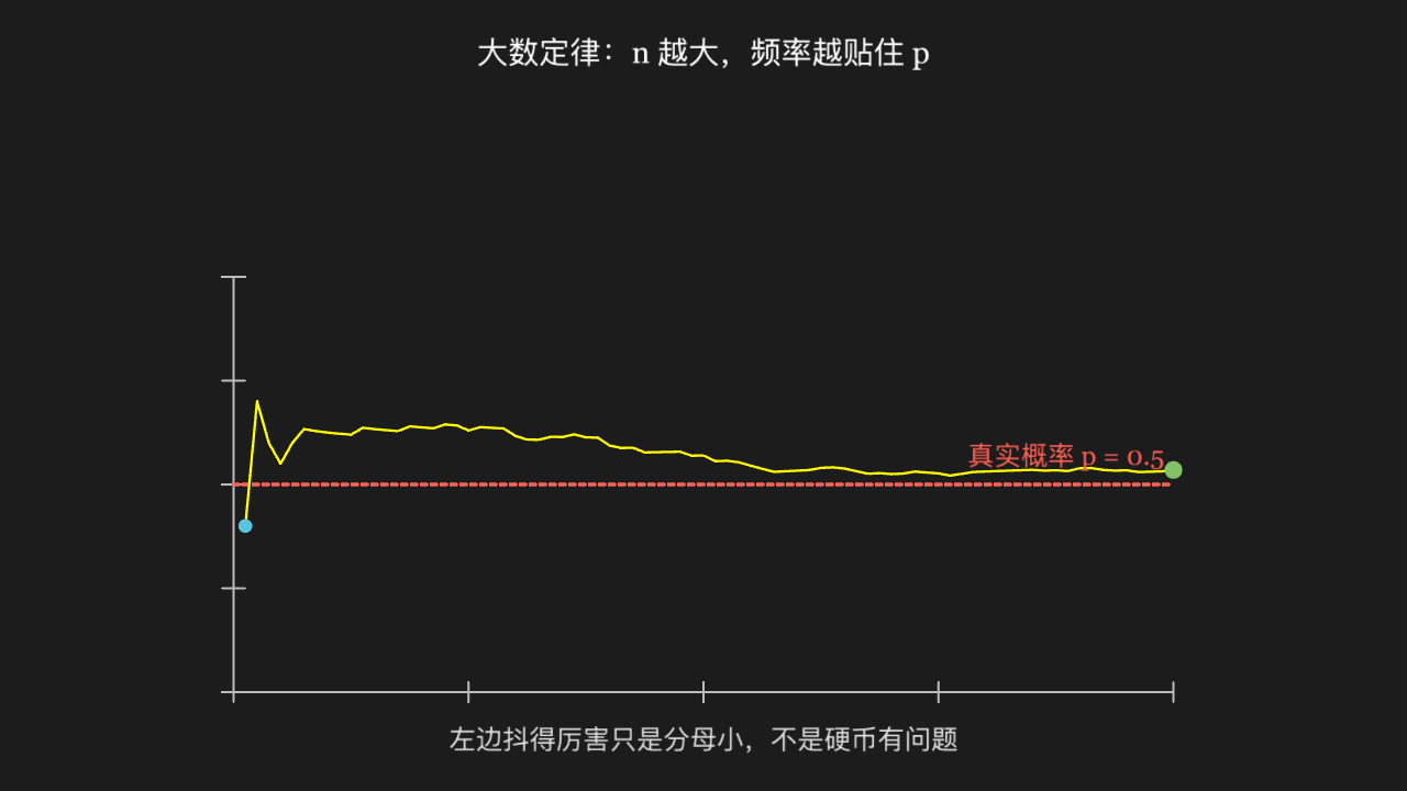
"""大数定律:频率随试验次数增加而贴向真实概率

@expect 一条从剧烈上下抖动开始、越往右摆幅越小的折线,逐渐收拢到 y=0.5 那条理论概率的虚线上——收敛是「以概率 1」的,不是每一步都单调靠近。
@note 讲解要点:折线在左侧跳得厉害并不代表不公平;大数定律说的是 n 趋于无穷时频率依概率收敛到 p。前几步的偏差会被庞大的分母稀释掉。
"""

from manim import *
import numpy as np


class LawOfLargeNumbersScene(Scene):
    def construct(self):
        rng = np.random.default_rng(2024)
        n_max = 400
        flips = (rng.random(n_max) < 0.5).astype(float)
        freq = np.cumsum(flips) / np.arange(1, n_max + 1)

        ax = Axes(
            x_range=[0, 400, 100],
            y_range=[0, 1, 0.25],
            x_length=9.5,
            y_length=4.2,
            tips=False,
            axis_config={"color": GRAY_B},
        )
        ax.shift(DOWN * 0.9)

        true_line = DashedLine(ax.c2p(0, 0.5), ax.c2p(400, 0.5), color=RED)
        true_label = Text("真实概率 p = 0.5", font_size=26, color=RED)
        true_label.next_to(true_line, UP, buff=0.12).align_to(true_line, RIGHT)

        step = 5
        pts = [ax.c2p(n, float(freq[n - 1])) for n in range(step, n_max + 1, step)]
        path = VGroup(
            *[Line(pts[i], pts[i + 1], color=YELLOW, stroke_width=2.5) for i in range(len(pts) - 1)]
        )

        start_mark = Dot(pts[0], radius=0.07, color=BLUE)
        end_mark = Dot(pts[-1], radius=0.09, color=GREEN)

        title = Text("大数定律:n 越大,频率越贴住 p", font_size=30).to_edge(UP, buff=0.35)
        caption = Text("左边抖得厉害只是分母小,不是硬币有问题", font_size=26, color=GRAY_A)
        caption.to_edge(DOWN, buff=0.35)

        self.play(Create(ax), Write(title), run_time=1.0)
        self.play(Create(true_line), Write(true_label), run_time=0.6)
        self.play(Create(path), FadeIn(start_mark), run_time=2.4, rate_func=linear)
        self.play(FadeIn(end_mark), run_time=0.4)
        self.play(Write(caption), run_time=0.7)
        self.wait(0.4)
Central limit theorem: sums of i.i.d. variables approach the normal shape
Three histograms side by side: one die (flat), the sum of two (triangular), the sum of four (clearly bell-shaped); the right two pile towards the middle with collapsing tails, normalized to equal height so the shapes compare.
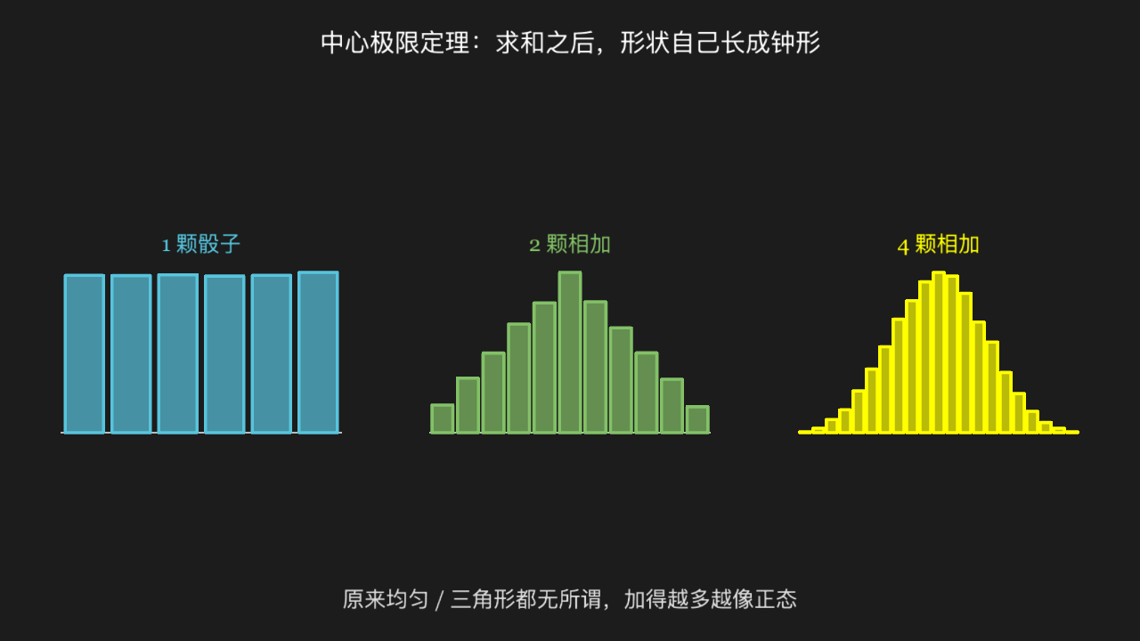
"""中心极限定理:独立同分布求和,分布形状必然向正态靠拢

@expect 三个并排直方图,从左到右分别是一颗骰子(平的)、两颗之和(三角形)、四颗之和(明显钟形);右侧两张的柱子朝中间堆、两端塌下去,且被归一化成同高以便比较形状。
@note 讲解要点:单颗骰子是完全均匀的,一点都不「正态」;但只要把若干独立同分布的变量加起来,中心就会长出钟形——不管原来是什么分布。这是正态分布无处不在的根源。
"""

from manim import *
import numpy as np


class CentralLimitScene(Scene):
    def construct(self):
        rng = np.random.default_rng(2026)
        samples = 20000

        def heights_for(k):
            rolls = rng.integers(1, 7, size=(samples, k)).sum(axis=1).tolist()
            counts = [0] * (6 * k - k + 1)
            for value in rolls:
                counts[value - k] += 1
            peak = max(counts)
            return [c / peak for c in counts]

        def make_panel(k, center, color):
            hs = heights_for(k)
            span = 3.5
            slot = span / len(hs)
            bars = VGroup()
            for i, h in enumerate(hs):
                bar = Rectangle(width=slot * 0.82, height=float(h) * 2.0, color=color)
                bar.set_fill(color, opacity=0.7)
                bar.move_to([center - span / 2 + slot * (i + 0.5), -1.4 + float(h), 0])
                bars.add(bar)
            return bars

        panel_cfg = [(1, -4.6, BLUE, "1 颗骰子"), (2, 0.0, GREEN, "2 颗相加"), (4, 4.6, YELLOW, "4 颗相加")]
        bars_all = VGroup()
        titles = VGroup()
        for k, center, color, name in panel_cfg:
            bars_all.add(make_panel(k, center, color))
            titles.add(Text(name, font_size=26, color=color).move_to([center, 0.95, 0]))

        baseline = VGroup(
            *[Line([c - 1.75, -1.4, 0], [c + 1.75, -1.4, 0], color=GRAY_B, stroke_width=2) for _, c, _, _ in panel_cfg]
        )

        title = Text("中心极限定理:求和之后,形状自己长成钟形", font_size=30).to_edge(UP, buff=0.35)
        caption = Text(
            "原来均匀 / 三角形都无所谓,加得越多越像正态",
            font_size=26,
            color=GRAY_A,
        ).to_edge(DOWN, buff=0.35)

        self.play(Write(title), Create(baseline), run_time=0.8)
        self.play(LaggedStart(*[FadeIn(p) for p in bars_all], lag_ratio=0.25), run_time=2.0)
        self.play(Write(titles), run_time=0.8)
        self.play(Write(caption), run_time=0.7)
        self.wait(0.4)
Poisson distribution: rare-event arrivals on a time axis
Arrival times scattered unevenly along a time axis (events cannot overlap), beside the count distribution bars: highest around k=2, 3 and decaying fast at both ends.
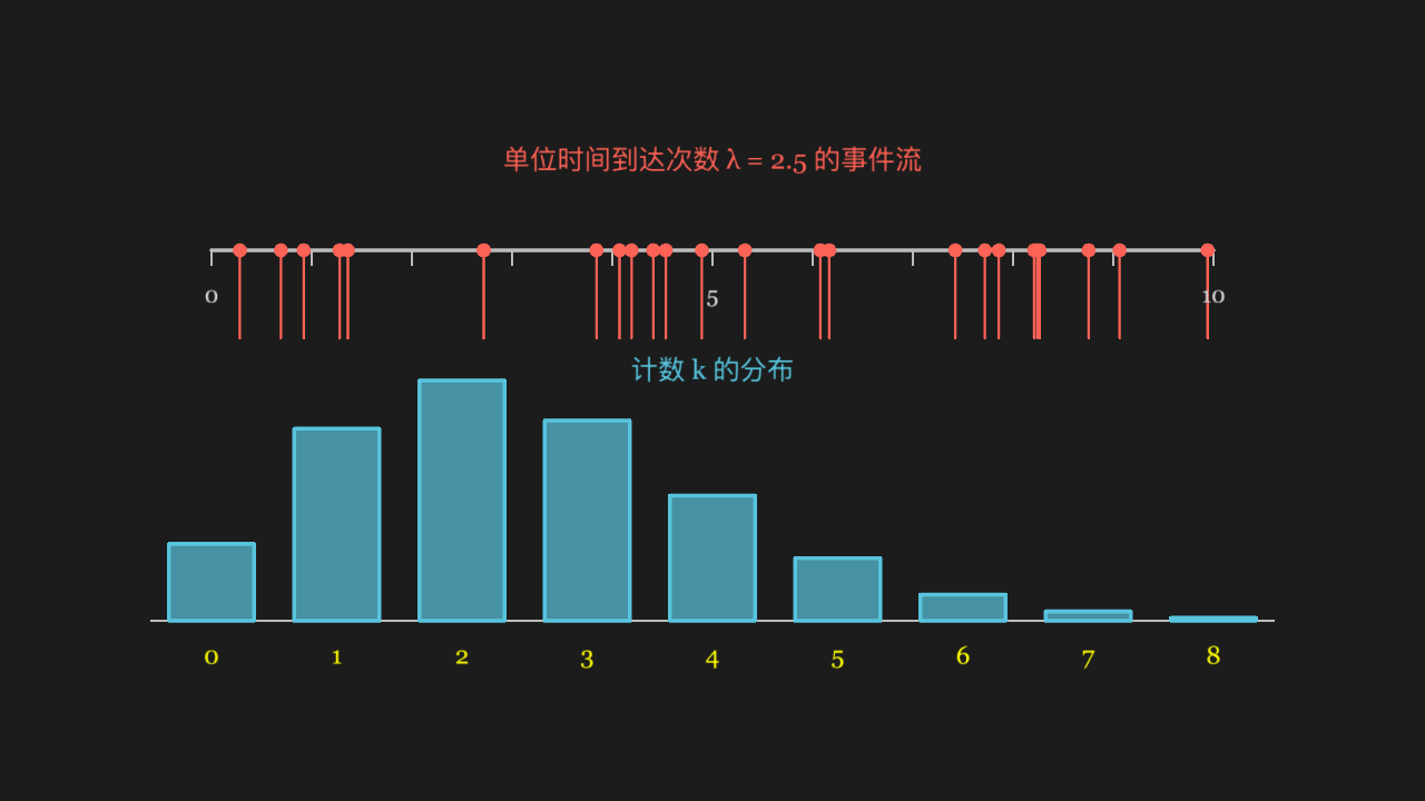
"""泊松分布:稀有事件在时间轴上的到达

@expect 一条时间轴上不均匀地散落着若干次到达时刻(事件不能重叠),旁边画出计数 k 的分布柱:k=2、3 附近最高,两端迅速衰减。
@note 讲解要点:泊松过程描述「单位时间内随机到达的稀有事件」——到达是独立的、速率恒定,于是计数服从泊松分布,它的期望和方差都等于 λ。
"""

from manim import *
import math
import numpy as np


class PoissonArrivalsScene(Scene):
    def construct(self):
        lam = 2.5
        length = 10.0
        rng = np.random.default_rng(7)

        gaps = rng.exponential(1.0 / lam, size=60)
        arrivals = np.cumsum(gaps)
        # 时间窗 [0, length] 线性映到数轴 [-5, 5]
        arrivals = arrivals[arrivals < length] - 5.0

        timeline = Line([-5.0, 1.5, 0], [5.0, 1.5, 0], color=GRAY_B, stroke_width=4)
        tick_labels = VGroup()
        for i in range(11):
            x = -5.0 + i
            tick_labels.add(Line([x, 1.5, 0], [x, 1.35, 0], color=GRAY_B, stroke_width=2))
            if i % 5 == 0:
                tick_labels.add(Text(str(i), font_size=22, color=GRAY_A).move_to([x, 1.05, 0]))

        drops = VGroup(
            *[
                Line([float(t), 1.5, 0], [float(t), 0.62, 0], color=RED, stroke_width=2.5) for t in arrivals
            ]
        )
        heads = VGroup(*[Dot([float(t), 1.5, 0], radius=0.07, color=RED) for t in arrivals])

        timeline_label = Text(f"单位时间到达次数 λ = {lam} 的事件流", font_size=26, color=RED)
        timeline_label.move_to([0, 2.4, 0])

        ks = list(range(0, 9))
        pmf = [float(np.exp(-lam) * lam ** k / math.factorial(k)) for k in ks]
        peak = max(pmf)
        bars = VGroup()
        labels_k = VGroup()
        for k, p in zip(ks, pmf):
            x = -5.0 + k * 1.25
            bar = Rectangle(width=0.85, height=p / peak * 2.4, color=BLUE)
            bar.set_fill(BLUE, opacity=0.7)
            bar.move_to([x, -2.2 + p / peak * 2.4 / 2, 0])
            bars.add(bar)
            labels_k.add(Text(str(k), font_size=24, color=YELLOW).move_to([x, -2.55, 0]))

        bar_axis = Line([-5.6, -2.2, 0], [5.6, -2.2, 0], color=GRAY_B, stroke_width=2)
        bar_label = Text("计数 k 的分布", font_size=26, color=BLUE).move_to([0, 0.3, 0])

        self.play(Write(timeline_label), Create(timeline), Create(tick_labels), run_time=0.9)
        self.play(LaggedStart(*[Create(d) for d in drops], lag_ratio=0.08), run_time=1.6)
        self.play(FadeIn(heads), run_time=0.5)
        self.play(Create(bar_axis), Write(bar_label), run_time=0.7)
        self.play(LaggedStart(*[FadeIn(b) for b in bars], lag_ratio=0.1), run_time=1.4)
        self.play(Write(labels_k), run_time=0.7)
        self.wait(0.4)
The 3σ rule of the normal distribution: how the area under the bell splits
Dashed cuts at ±1σ, ±2σ and ±3σ under the bell with the covered areas listed on the right; below, 1000 sample dots crowd the middle and the few beyond ±2.5σ are coloured red.
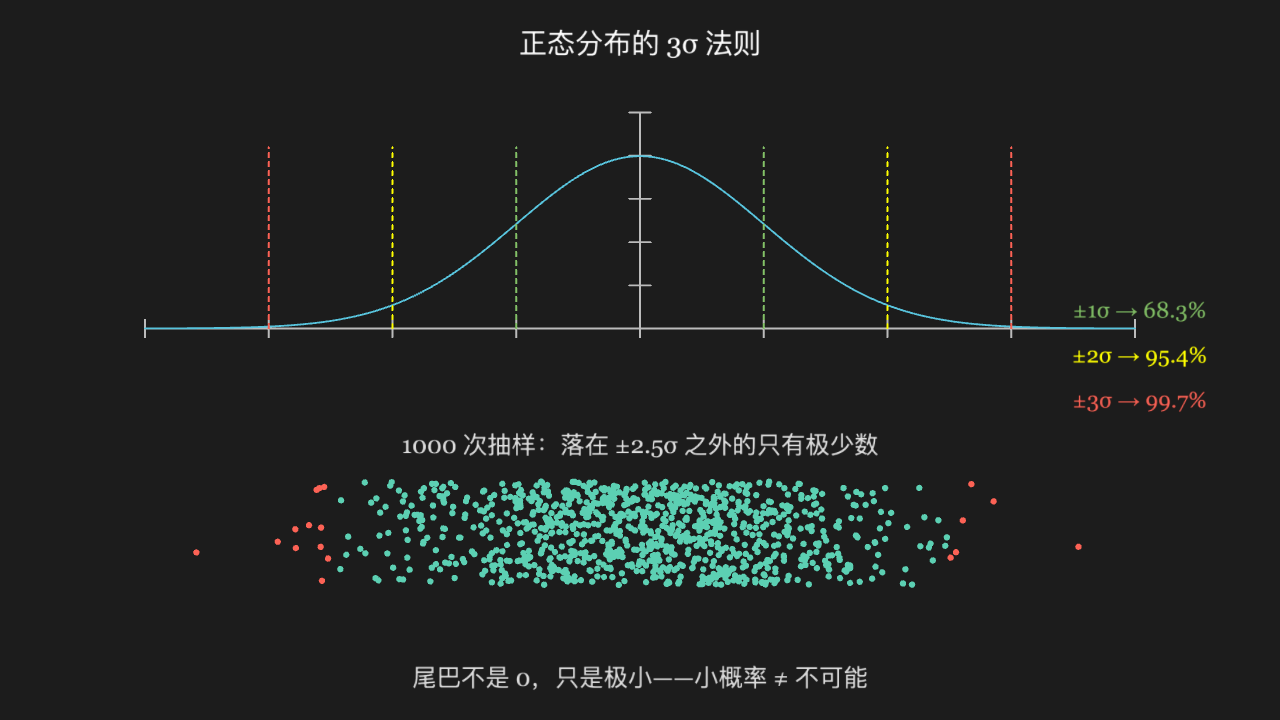
"""正态分布的 3σ 法则:钟形曲线下的面积怎么分

@expect 钟形曲线下方用虚线切出 ±1σ、±2σ、±3σ 三道关口,右侧列出各自覆盖的面积;下方 1000 次抽样的小点密密麻麻挤在中间,落在 ±2.5σ 之外的少数几个被染红。
@note 讲解要点:68.3% / 95.4% / 99.7% 说的是「概率集中在中心」,不是「值域到此为止」——尾巴永远存在,只是以小概率存在,所以 3σ 外的事件叫「小概率」而不叫「不可能」。
"""

from manim import *
import numpy as np


class NormalSigmaScene(Scene):
    def construct(self):
        rng = np.random.default_rng(31)
        pdf = lambda x: np.exp(-x * x / 2.0) / np.sqrt(2.0 * np.pi)

        ax = Axes(
            x_range=[-4, 4, 1],
            y_range=[0, 0.5, 0.1],
            x_length=11.0,
            y_length=2.4,
            tips=False,
            axis_config={"color": GRAY_B},
        )
        ax.shift(UP * 1.55)

        curve = ax.plot(lambda t: float(pdf(t)), x_range=[-4, 4], color=BLUE)

        gates = VGroup()
        for sigma, color in [(1.0, GREEN), (2.0, YELLOW), (3.0, RED)]:
            for sign in (-1, 1):
                gates.add(
                    DashedLine(
                        ax.c2p(sign * sigma, 0),
                        ax.c2p(sign * sigma, 0.42),
                        color=color,
                        stroke_width=2,
                    )
                )

        label_rows = VGroup(
            Text("±1σ → 68.3%", font_size=24, color=GREEN).move_to([5.55, 0.55, 0]),
            Text("±2σ → 95.4%", font_size=24, color=YELLOW).move_to([5.55, 0.05, 0]),
            Text("±3σ → 99.7%", font_size=24, color=RED).move_to([5.55, -0.45, 0]),
        )

        raw = rng.normal(0.0, 1.0, size=1000)
        ys = rng.uniform(-2.5, -1.35, size=1000)
        inside = VGroup()
        outside = VGroup()
        for value, y in zip(raw, ys):
            # 抽样点的 x 要过 c2p 换算,才和上方曲线同一个比例
            px = ax.c2p(float(value), 0)[0]
            if abs(value) > 2.5:
                outside.add(Dot([px, float(y), 0], radius=0.035, color=RED))
            else:
                inside.add(Dot([px, float(y), 0], radius=0.035, color=TEAL))

        sample_note = Text("1000 次抽样:落在 ±2.5σ 之外的只有极少数", font_size=26, color=GRAY_A)
        sample_note.move_to([0, -0.95, 0])

        title = Text("正态分布的 3σ 法则", font_size=30).to_edge(UP, buff=0.3)
        caption = Text("尾巴不是 0,只是极小——小概率 ≠ 不可能", font_size=26, color=GRAY_A)
        caption.to_edge(DOWN, buff=0.3)

        self.play(Write(title), Create(ax), run_time=0.8)
        self.play(Create(curve), run_time=1.2)
        self.play(Create(gates), Write(label_rows), run_time=1.0)
        self.play(LaggedStart(*[FadeIn(d) for d in inside], lag_ratio=0.002), run_time=1.6)
        self.play(FadeIn(outside), Write(sample_note), run_time=0.8)
        self.play(Write(caption), run_time=0.7)
        self.wait(0.4)
Monte Carlo estimate of π: scatter points and count those inside the quarter circle
A quarter circle inside a square of side 2 with blue points scattered at random: those inside the arc turn yellow, the rest stay blue; the bottom-right readout shows the running ratio times 4 approaching 3.14.
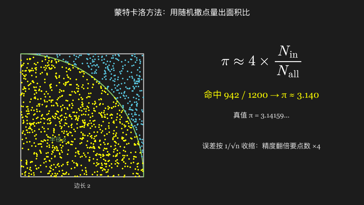
"""蒙特卡洛估算 π:往正方形里撒点,数落在四分之一圆内的比例

@expect 边长为 2 的正方形内含一个四分之一圆,蓝点在正方形里随机撒开:落在圆弧内的染黄、在外面的留蓝;右下角实时显示累计比例乘 4 逼近 3.14。
@note 讲解要点:P(落在圆内) = 圆面积/正方形面积 = π/4,所以 π ≈ 4 × 命中比例。随机模拟的误差按 1/√n 收缩,想把精度翻倍就得撒四倍的点。
"""

from manim import *
import numpy as np


class MonteCarloPiScene(Scene):
    def construct(self):
        rng = np.random.default_rng(1024)
        radius = 2.4
        # 圆心(四分之一圆的圆心在正方形左下角)
        cx, cy = -3.9, -0.5
        x0, y0 = cx + radius, cy + radius

        square = Rectangle(width=2 * radius, height=2 * radius, color=GRAY_B)
        square.move_to([cx, cy, 0])
        # 四分之一圆的半径 = 正方形边长(圆心在左下角,弧端点落在另外两个角上)。
        # Arc 以圆心为原点生成,shift 直接把圆心放到左下角——不能用 move_to(那挪的是外接框中心)
        arc = Arc(radius=2 * radius, start_angle=0, angle=PI / 2, color=GREEN, stroke_width=4)
        arc.shift([cx - radius, cy - radius, 0])

        side_label = Text("边长 2", font_size=22, color=GRAY_A).move_to([cx, cy - radius - 0.35, 0])
        # 标签沿弧的 45° 方向放在弧内,别压在点堆里
        arc_label = Text("半径 2", font_size=22, color=GREEN).move_to(
            [cx - radius + 1.45, cy - radius + 1.45, 0]
        )

        pts = rng.random((1200, 2))
        hits = VGroup()
        misses = VGroup()
        for u, v in pts:
            x = cx - radius + float(u) * 2 * radius
            y = cy - radius + float(v) * 2 * radius
            if u * u + v * v <= 1.0:
                hits.add(Dot([x, y, 0], radius=0.03, color=YELLOW))
            else:
                misses.add(Dot([x, y, 0], radius=0.03, color=BLUE))

        ratio = len(hits) / len(pts)
        estimate = 4.0 * ratio

        formula = MathTex(
            r"\pi \approx 4 \times \frac{N_{\text{in}}}{N_{\text{all}}}",
            font_size=54,
        ).move_to([3.1, 1.6, 0])

        result = Text(f"命中 {len(hits)} / {len(pts)} → π ≈ {estimate:.3f}", font_size=34, color=YELLOW)
        result.move_to([3.1, 0.3, 0])
        truth = Text("真值 π = 3.14159...", font_size=26, color=GRAY_A).move_to([3.1, -0.5, 0])

        error_note = Text("误差按 1/√n 收缩:精度翻倍要点数 ×4", font_size=26, color=GRAY_A)
        error_note.move_to([3.1, -1.7, 0])

        title = Text("蒙特卡洛方法:用随机撒点量出面积比", font_size=30).to_edge(UP, buff=0.3)

        self.play(Write(title), run_time=0.7)
        self.play(Create(square), Create(arc), Write(side_label), Write(arc_label), run_time=0.9)
        self.play(LaggedStart(*[FadeIn(d) for d in hits], lag_ratio=0.01), run_time=1.6)
        self.play(FadeIn(misses), run_time=0.8)
        self.play(Write(formula), run_time=0.8)
        self.play(Write(result), Write(truth), run_time=0.8)
        self.play(Write(error_note), run_time=0.7)
        self.wait(0.4)
Random walk: memoryless steps, yet a √n scale overall
Four independent one-dimensional walks leave the origin together, each wandering out of sync; the endpoints are marked and the horizontal envelope around them is far narrower than the step count — the typical scale is √n, not n.
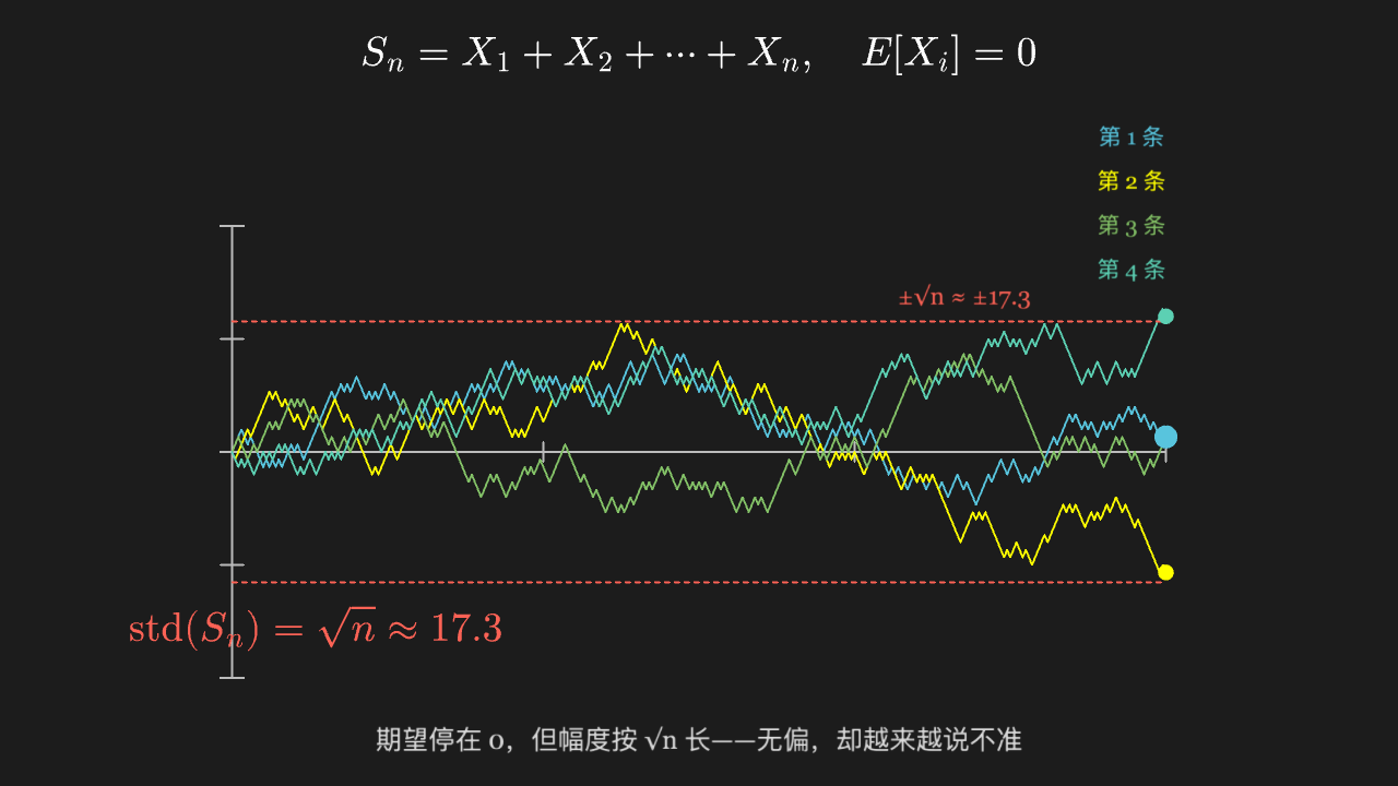
"""随机游走:每一步无记忆,但整体呈现出 √n 的尺度

@expect 四条独立的一维随机游走轨迹同时从原点出发,各自上下乱走、互不同步;终点被标出,包围它们的横向包络宽度远小于步数——典型量级是 √n 而不是 n。
@note 讲解要点:每一步的期望位移是 0,所以游走不会「漂」到某一边;但方差逐步累加,标准差按 √n 增长。这正是「无偏但不确定」的标准图像,也是扩散方程与布朗运动的离散原型。
"""

from manim import *
import numpy as np
import math


class RandomWalkScene(Scene):
    def construct(self):
        rng = np.random.default_rng(1234)
        steps = 300
        colors = [BLUE, YELLOW, GREEN, TEAL]

        ax = Axes(
            x_range=[0, 300, 100],
            y_range=[-30, 30, 15],
            x_length=9.5,
            y_length=4.6,
            tips=False,
            axis_config={"color": GRAY_B},
        )
        ax.shift(DOWN * 0.6)

        zero_line = DashedLine(ax.c2p(0, 0), ax.c2p(300, 0), color=GRAY_B, stroke_width=2)

        # ±√n 参考带:两端绝对坐标(c2p),直观对照「包络宽度 ~ √n 而非 n」
        sqrt_n = math.sqrt(300)
        band_top = DashedLine(ax.c2p(0, sqrt_n), ax.c2p(300, sqrt_n), color=RED, stroke_width=2)
        band_bottom = DashedLine(ax.c2p(0, -sqrt_n), ax.c2p(300, -sqrt_n), color=RED, stroke_width=2)
        band_label = Text("±√n ≈ ±17.3", font_size=24, color=RED).move_to([2.7, 0.98, 0])

        walks = VGroup()
        ends = VGroup()
        legend = VGroup()
        end_pts = []
        for idx, color in enumerate(colors):
            moves = rng.choice([-1.0, 1.0], size=steps)
            path_values = np.concatenate([[0.0], np.cumsum(moves)])
            pts = [ax.c2p(int(i), float(v)) for i, v in enumerate(path_values)]
            walks.add(
                VGroup(*[Line(pts[i], pts[i + 1], color=color, stroke_width=2) for i in range(len(pts) - 1)])
            )
            end_pts.append(pts[-1])
            ends.add(Dot(pts[-1], radius=0.08, color=color))
            legend.add(Text(f"第 {idx + 1} 条", font_size=22, color=color).move_to([4.4, 2.6 - idx * 0.45, 0]))
        # 蓝色终点单独补一颗稍大的点,避免与其他终点重叠后看不见
        blue_end_dot = Dot(end_pts[0], radius=0.11, color=BLUE, stroke_color=WHITE, stroke_width=1.5)

        sigma_note = MathTex(r"\text{std}(S_n) = \sqrt{n} \approx 17.3", font_size=40, color=RED)
        sigma_note.move_to([-3.9, -2.4, 0])
        formula = MathTex(r"S_n = X_1 + X_2 + \cdots + X_n,\quad E[X_i] = 0", font_size=40)
        formula.to_edge(UP, buff=0.35)
        caption = Text("期望停在 0,但幅度按 √n 长——无偏,却越来越说不准", font_size=26, color=GRAY_A)
        caption.to_edge(DOWN, buff=0.3)

        self.play(Write(formula), run_time=0.8)
        self.play(Create(ax), Create(zero_line), run_time=0.9)
        self.play(LaggedStart(*[Create(w) for w in walks], lag_ratio=0.3), run_time=3.0)
        self.play(FadeIn(ends), FadeIn(blue_end_dot), Write(legend), run_time=0.7)
        self.play(Create(band_top), Create(band_bottom), Write(band_label), run_time=0.8)
        self.play(Write(sigma_note), run_time=0.7)
        self.play(Write(caption), run_time=0.7)
        self.wait(0.4)
The two errors of hypothesis testing: α rejects the true, β accepts the false
Two offset bell curves stand for H0 and H1; H0's right tail is cut into a red region (type I / false positive) and H1's left tail into a yellow region (type II / false negative), with the vertical line between them as the rejection threshold.
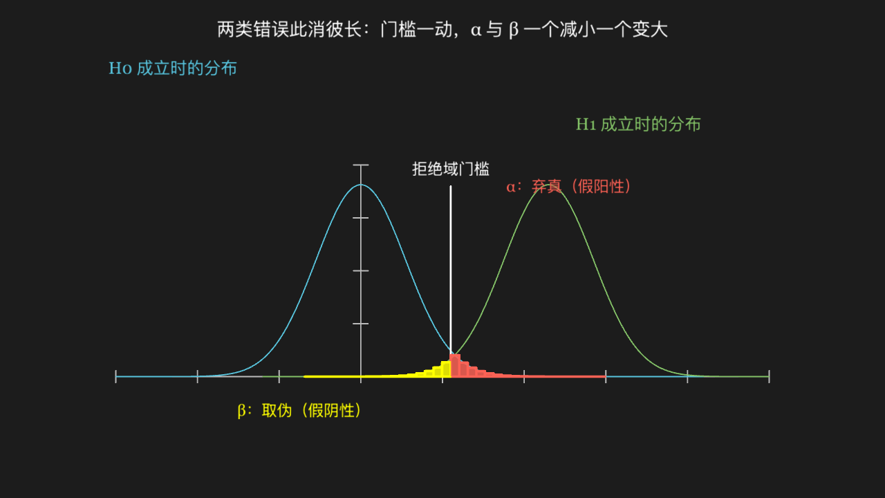
"""假设检验的两类错误:α 是弃真,β 是取伪

@expect 两条错开的钟形曲线分别代表原假设 H0 与备择假设 H1;H0 右尾被切出红线区(弃真 / 假阳性),H1 左尾被切出黄线区(取伪 / 假阴性),中间那道竖线就是拒绝域的门槛。
@note 讲解要点:门槛往右移,弃真概率 α 变小、但取伪概率 β 变大;两者此消彼长,不可能同时压到最低。只有加大样本量让两条曲线变瘦,才能同时把 α 和 β 都收小。
"""

from manim import *
import numpy as np


class HypothesisTestScene(Scene):
    def construct(self):
        pdf = lambda x, mu: np.exp(-(x - mu) ** 2 / (2 * 0.55 ** 2)) / (0.55 * np.sqrt(2 * np.pi))

        ax = Axes(
            x_range=[-3, 5, 1],
            y_range=[0, 0.8, 0.2],
            x_length=10.5,
            y_length=3.4,
            tips=False,
            axis_config={"color": GRAY_B},
        )
        ax.shift(DOWN * 0.35)

        critical = 1.1
        h0_mu = 0.0
        h1_mu = 2.3

        curve_h0 = ax.plot(lambda t: float(pdf(t, h0_mu)), x_range=[-3, 4.2], color=BLUE)
        curve_h1 = ax.plot(lambda t: float(pdf(t, h1_mu)), x_range=[-1.2, 5], color=GREEN)

        bar_span = (critical + 4.2) - critical
        bar_w = bar_span / 40.0
        alpha_bars = VGroup()
        for i in range(40):
            x = critical + bar_w * (i + 0.5)
            y_low = ax.c2p(0, 0)[1]
            y_high = ax.c2p(0, float(pdf(x, h0_mu)))[1]
            if abs(y_high - y_low) < 1e-6:
                continue
            bar = Rectangle(width=abs(ax.c2p(bar_w, 0)[0] - ax.c2p(0, 0)[0]), height=y_high - y_low, color=RED)
            bar.set_fill(RED, opacity=0.85)
            bar.move_to([ax.c2p(x, 0)[0], (y_low + y_high) / 2, 0])
            alpha_bars.add(bar)

        beta_bars = VGroup()
        for i in range(40):
            x = critical - bar_w * (i + 0.5)
            y_low = ax.c2p(0, 0)[1]
            y_high = ax.c2p(0, float(pdf(x, h1_mu)))[1]
            if abs(y_high - y_low) < 1e-6:
                continue
            bar = Rectangle(width=abs(ax.c2p(bar_w, 0)[0] - ax.c2p(0, 0)[0]), height=y_high - y_low, color=YELLOW)
            bar.set_fill(YELLOW, opacity=0.85)
            bar.move_to([ax.c2p(x, 0)[0], (y_low + y_high) / 2, 0])
            beta_bars.add(bar)

        gate = Line(ax.c2p(critical, 0), ax.c2p(critical, 0.72), color=WHITE, stroke_width=3)
        gate_label = Text("拒绝域门槛", font_size=24, color=WHITE).next_to(gate, UP, buff=0.12)

        labels = VGroup(
            Text("H0 成立时的分布", font_size=26, color=BLUE).move_to([ax.c2p(-2.3, 0)[0], 2.9, 0]),
            Text("H1 成立时的分布", font_size=26, color=GREEN).move_to([ax.c2p(3.4, 0)[0], 2.0, 0]),
            Text("α:弃真(假阳性)", font_size=24, color=RED).move_to([ax.c2p(2.6, 0)[0], 1.0, 0]),
            Text("β:取伪(假阴性)", font_size=24, color=YELLOW).move_to([ax.c2p(-0.7, 0)[0], -2.6, 0]),
        )

        title = Text("两类错误此消彼长:门槛一动,α 与 β 一个减小一个变大", font_size=28)
        title.to_edge(UP, buff=0.3)

        self.play(Write(title), Create(ax), run_time=0.8)
        self.play(Create(curve_h0), Create(curve_h1), run_time=1.4)
        self.play(Write(labels[0]), Write(labels[1]), run_time=0.7)
        self.play(Create(gate), Write(gate_label), run_time=0.6)
        self.play(FadeIn(alpha_bars), Write(labels[2]), run_time=0.9)
        self.play(FadeIn(beta_bars), Write(labels[3]), run_time=0.9)
        self.wait(0.4)