Lesson scenes (templates)
Reusable lesson patterns: unit circle, sine-wave tracing, Pythagoras, polar curves, secant-to-tangent, Riemann sums, linear maps and probability comparisons.
This page lists 13 examples. The code is imported from corpus/examples/lesson/; the screenshots are end states rendered on real machines.
Unit circle and trigonometric lines
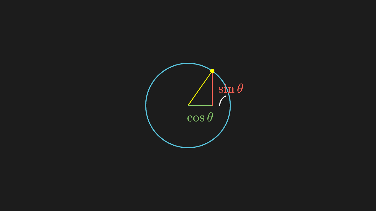
A point travels on the unit circle while the sine / cosine lines stretch with the angle; their lengths match the angle.
"""单位圆与三角函数线

@expect 单位圆上一点转动,正弦 / 余弦线随角度伸缩,长度与角度对得上。
@template 要画「一个量随角度/参数变化」的静态定义图(圆上取点 + 投影线 + 对应公式标注)时照它抄。
@note 讲解模板:角度 → 圆上一点 → sin / cos 两条投影线。讲定义的静态图
"""

from manim import *
import numpy as np


class UnitCircleScene(Scene):
    def construct(self):
        radius = 1.6
        angle = 55 * DEGREES
        point = np.array([radius * np.cos(angle), radius * np.sin(angle), 0])

        circle = Circle(radius=radius, color=BLUE)
        radius_line = Line(start=ORIGIN, end=point, color=YELLOW)
        cos_leg = Line(start=ORIGIN, end=[point[0], 0, 0], color=GREEN)
        sin_leg = Line(start=[point[0], 0, 0], end=point, color=RED)
        dot = Dot(point=point, radius=0.08, color=YELLOW)
        arc = Angle([[0, 0, 0], [radius, 0, 0], point], radius=0.4)
        label_cos = MathTex(r"\cos\theta", color=GREEN).next_to(cos_leg, DOWN)
        label_sin = MathTex(r"\sin\theta", color=RED).next_to(sin_leg, RIGHT)

        self.play(Create(circle))
        self.play(Create(radius_line), FadeIn(dot), Create(arc))
        self.play(Create(cos_leg), Write(label_cos))
        self.play(Create(sin_leg), Write(label_sin))
        self.wait(0.3)
Tracing a sine wave from a point on the circle
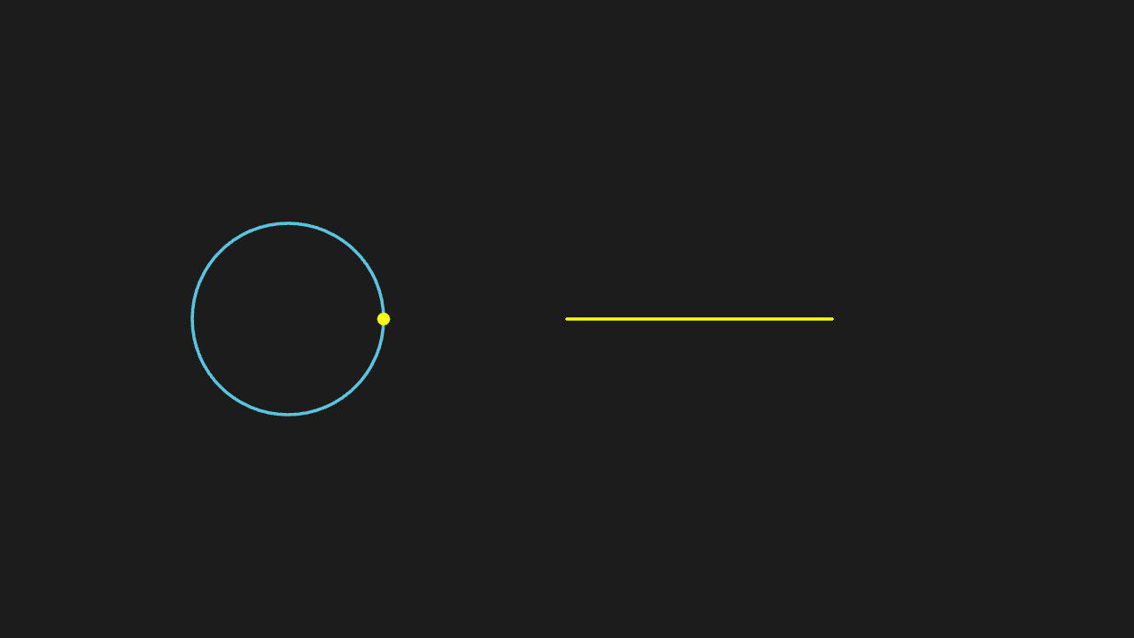
As the point on the circle turns, the wave unfolds to the right and what is drawn is exactly the sine curve (a full sine of amplitude ±1.2, observed in real time; with turbo screenshots the sparse frames can collapse a TracedPath trail into a straight line — a screenshot artefact).
"""从圆上一点画出正弦波

@expect 圆上的点一边转、波形一边向右展开,画出的正是正弦曲线(振幅 ±1.2 的完整正弦,真时序下观察;极速截图帧点过疏会让 TracedPath 轨迹塌成直线,属截图假象)。
@template 要让一个点/量被 ValueTracker 驱动、边动边扫出轨迹(TracedPath / updaters)时照它抄。
@note 讲解模板:ValueTracker 驱动圆上的点,TracedPath 把它的高度扫成波形;留存截图用 --realtime 真时序重截
"""

from manim import *
import numpy as np


class SineWaveScene(Scene):
    def construct(self):
        radius = 1.2
        circle = Circle(radius=radius, color=BLUE).shift(LEFT * 3.5)
        dot = Dot(radius=0.08, color=YELLOW)
        pen = Dot(radius=0.001)
        wave = TracedPath(pen, stroke_color=YELLOW)
        tracker = ValueTracker(0)

        def follow(mob):
            angle = tracker.get_value()
            dot.move_to([-3.5 + radius * np.cos(angle), radius * np.sin(angle), 0])
            pen.move_to([0.5 + angle * 0.45, radius * np.sin(angle), 0])

        dot.add_updater(follow)
        pen.add_updater(follow)
        self.add(circle, wave, dot, pen)
        self.play(tracker.animate.set_value(TAU), run_time=3)
        self.wait(0.3)
The Pythagorean theorem
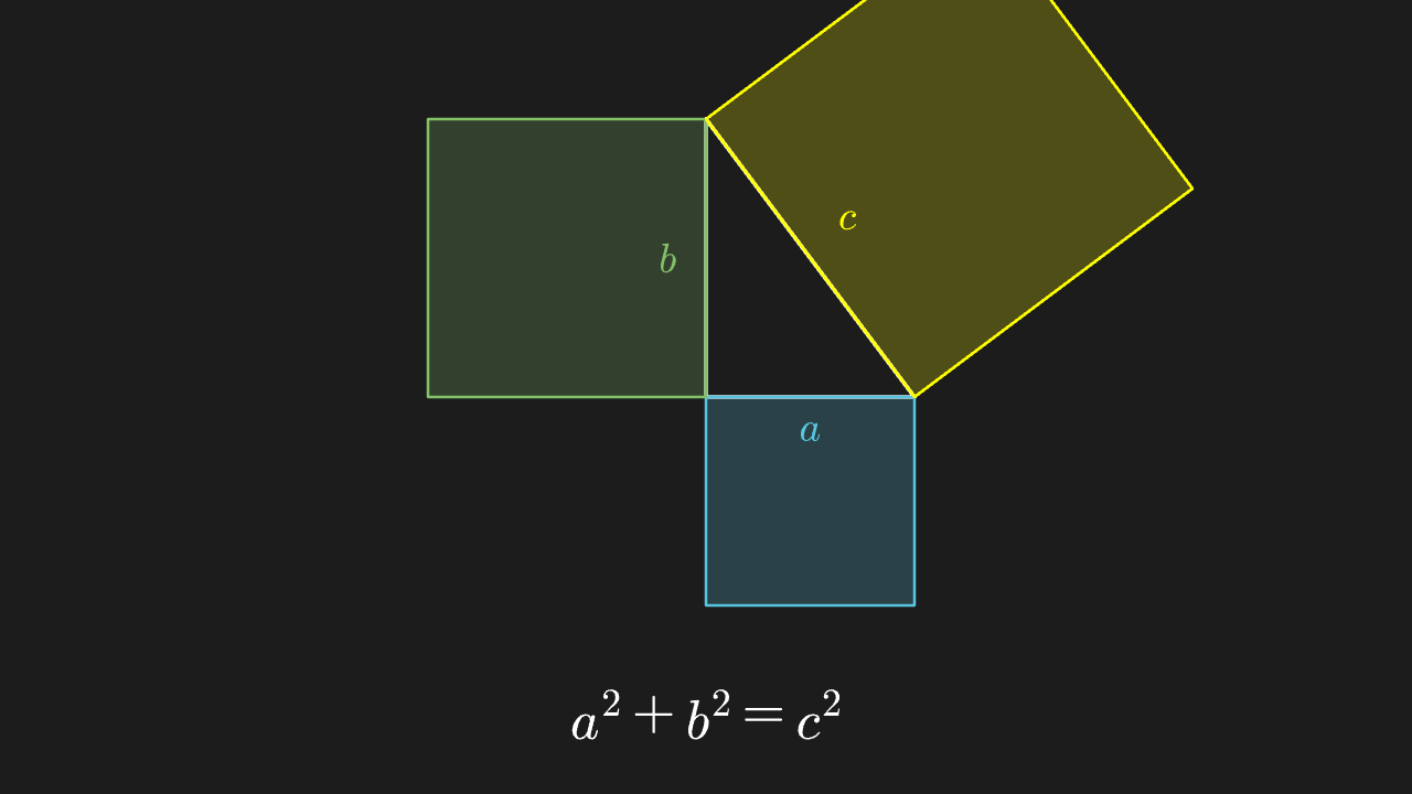
Squares on the three sides of a right triangle present the area relation a² + b² = c².
"""勾股定理

@expect 直角三角形三边上贴的正方形面积关系呈现 a² + b² = c²。
@note 讲解模板:直角三角形 + 两条直角边上的正方形,公式在下方
"""

from manim import *
import numpy as np


class PythagoreanScene(Scene):
    def construct(self):
        s = 0.7
        A = np.array([0.0, 0.0, 0.0])
        B = A + RIGHT * (3 * s)
        C = A + UP * (4 * s)

        triangle = Polygon(A, B, C, color=WHITE, stroke_width=4)
        a_label = MathTex("a", font_size=40, color=BLUE).move_to((A + B) / 2 + DOWN * 0.35)
        b_label = MathTex("b", font_size=40, color=GREEN).move_to((A + C) / 2 + LEFT * 0.38)
        c_label = MathTex("c", font_size=40, color=YELLOW).move_to((B + C) / 2 + UR * 0.38)

        sq_a = Polygon(A, B, B + DOWN * (3 * s), A + DOWN * (3 * s), color=BLUE, stroke_width=3)
        sq_a.set_fill(BLUE, 0.22)
        sq_b = Polygon(A, C, C + LEFT * (4 * s), A + LEFT * (4 * s), color=GREEN, stroke_width=3)
        sq_b.set_fill(GREEN, 0.22)
        offset = np.array([4 * s, 3 * s, 0.0])
        sq_c = Polygon(B, C, C + offset, B + offset, color=YELLOW, stroke_width=3)
        sq_c.set_fill(YELLOW, 0.22)

        shapes = VGroup(triangle, sq_a, sq_b, sq_c, a_label, b_label, c_label)
        shapes.shift(-shapes.get_center())

        eq = MathTex("a^2", "+", "b^2", "=", "c^2", font_size=54)
        eq.arrange(RIGHT, buff=0.16)
        eq.to_edge(DOWN, buff=0.55)

        self.play(Create(triangle), run_time=1.0)
        self.play(Write(a_label), Write(b_label), Write(c_label), run_time=0.6)
        self.play(Create(sq_a), Create(sq_b), run_time=1.0)
        self.play(Create(sq_c), run_time=1.0)
        self.play(Write(eq), run_time=0.8)
        self.play(Indicate(eq, color=WHITE, scale_factor=1.1), run_time=0.8)
        self.wait(0.5)
Polar rose curve
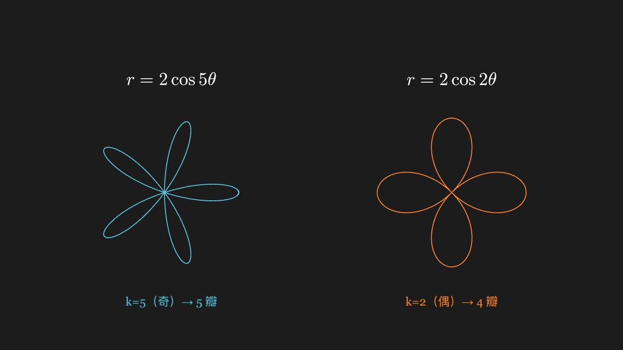
The petal count matches the equation parameters: left k=5 gives 5 petals (k odd), right k=2 gives 4 petals (2k petals, k even); each curve carries its equation label so the odd-k → k petals / even-k → 2k petals rule is readable by comparison.
"""极坐标玫瑰线

@expect 玫瑰线的花瓣数与方程参数一致:左边 k=5 是 5 瓣(k 奇)、右边 k=2 是 4 瓣(2k 瓣,k 偶),
两条曲线各自配方程标注,「奇 k → k 瓣 / 偶 k → 2k 瓣」的规律对照着看得出来。
@template 要画极坐标 / 参数方程曲线(玫瑰线、螺线、摆线……manim-web 没有 plot_polar_graph)时照它抄。
@note 讲解模板:manim-web 没有 plot_polar_graph——把 r(θ) 写成参数方程交给 ParametricFunction;
    MathTex 定位只能 move_to 绝对坐标(to_edge 会拿 NaN 包围盒把公式挪出画框)
"""

from manim import *
import numpy as np


class PolarRoseScene(Scene):
    def construct(self):
        def rose(petals, scale):
            def f(t):
                r = scale * np.cos(petals * t)
                return [r * np.cos(t), r * np.sin(t), 0]
            return f

        # 左:k=5(10 瓣);右:k=2(4 瓣)——两组并排对照
        curve_5 = ParametricFunction(rose(5, 1.7), t_range=[0, TAU, 0.02], color=BLUE)
        curve_5.move_to([-3.2, -0.4, 0])
        curve_2 = ParametricFunction(rose(2, 1.7), t_range=[0, TAU, 0.02], color=ORANGE)
        curve_2.move_to([3.2, -0.4, 0])

        title_5 = MathTex(r"r = 2\cos 5\theta", font_size=40).move_to([-3.2, 2.2, 0])
        title_2 = MathTex(r"r = 2\cos 2\theta", font_size=40).move_to([3.2, 2.2, 0])
        note_5 = Text("k=5(奇)→ 5 瓣", font_size=26, color=BLUE).move_to([-3.2, -2.9, 0])
        note_2 = Text("k=2(偶)→ 4 瓣", font_size=26, color=ORANGE).move_to([3.2, -2.9, 0])

        self.play(Write(title_5))
        self.play(Create(curve_5), FadeIn(note_5), run_time=2)
        self.play(Write(title_2))
        self.play(Create(curve_2), FadeIn(note_2), run_time=2)
        self.wait(0.3)
Archimedean spiral
The spiral widens turn by turn with a constant gap between turns (the defining trait of an Archimedean spiral).
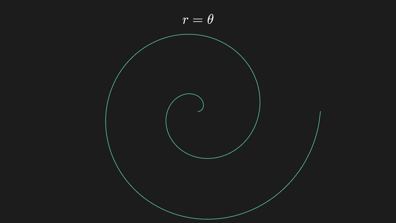
"""阿基米德螺线

@expect 螺线一圈圈等距外扩,圈距恒定(阿基米德螺线的特征)。
@note 讲解模板:r 随 θ 线性增长,同样用参数方程画
"""

from manim import *
import numpy as np


class PolarSpiralScene(Scene):
    def construct(self):
        def spiral(t):
            r = 0.35 * t
            return [r * np.cos(t), r * np.sin(t), 0]

        curve = ParametricFunction(spiral, t_range=[0, TAU * 2, 0.02], color=TEAL)
        title = MathTex(r"r = \theta").to_edge(UP)

        self.play(Write(title))
        self.play(Create(curve), run_time=2)
        self.wait(0.3)
Secants approaching the tangent (the definition of the derivative)
The secant rotates about the tangency point, hugging the tangent ever closer until they coincide.
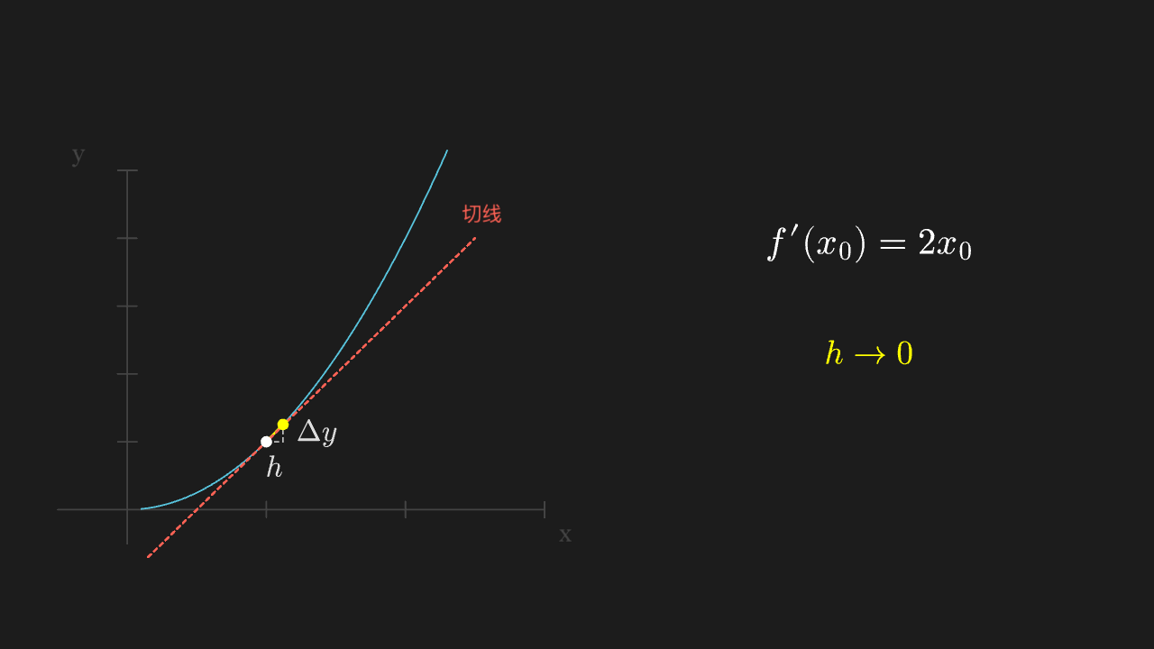
"""割线趋近切线(导数的定义)

@expect 割线绕切点旋转、越来越贴近切线,最终重合。
@template 要讲「极限 / 趋近」——一条线或一个量随参数滑动、逼近目标位置时照它抄。
@note 2026-10-09 真机事故原文:这段被预检误拒两次——`(pos_p() + pos_m()) / 2` 与
      `x0 + h.get_value()` 都拿 c2p / get_value 的返回值做算术,而预检把它们当成了 Mobject
      (`TypeError: unsupported operand type(s) for /: 'Mobject' and 'int'`)。
      修在支持面的 METHOD_RETURNS:预检按真桥的形状返值(坐标→向量、数值→数)。
"""

from manim import *
import numpy as np


class SecantToTangent(Scene):
    def construct(self):
        ax = Axes(
            x_range=[-0.5, 3, 1],
            y_range=[-0.5, 5, 1],
            x_length=6.0,
            y_length=4.6,
            tips=False,
            axis_config={"color": GRAY_D},
        )
        ax.shift(LEFT * 3.4 + DOWN * 0.4)
        # 轴标签手动定位:get_axis_labels 的自动定位会把 "x" 漂到轴外空白处;
        # 适配层 ax.x_axis 是函数不能 get_end,改用 c2p 手算轴末端坐标
        label_x = Text("x", font_size=30, color=GRAY_D).move_to(ax.c2p(3.15, -0.35))
        label_y = Text("y", font_size=30, color=GRAY_D).move_to(ax.c2p(-0.35, 5.25))

        graph = ax.plot(lambda x: x ** 2, x_range=[0.1, 2.3], color=BLUE)

        x0 = 1.0
        h = ValueTracker(1.0)

        def pos_p():
            return ax.c2p(x0, x0 ** 2, 0)

        def pos_q():
            x = x0 + h.get_value()
            return ax.c2p(x, x ** 2, 0)

        def pos_m():
            x = x0 + h.get_value()
            return ax.c2p(x, x0 ** 2, 0)

        # 割线
        secant = Line(pos_p(), pos_q(), color=YELLOW, stroke_width=3)
        secant.add_updater(lambda m: m.put_start_and_end_on(pos_p(), pos_q()))

        # 两点
        dot_p = Dot(pos_p(), color=WHITE, radius=0.07)
        dot_q = Dot(pos_q(), color=YELLOW, radius=0.07)
        dot_q.add_updater(lambda m: m.move_to(pos_q()))

        # 水平 / 竖直增量
        seg_dx = DashedLine(pos_p(), pos_m(), color=GRAY_B, stroke_width=2)
        seg_dx.add_updater(lambda m: m.put_start_and_end_on(pos_p(), pos_m()))
        seg_dy = DashedLine(pos_m(), pos_q(), color=GRAY_B, stroke_width=2)
        seg_dy.add_updater(lambda m: m.put_start_and_end_on(pos_m(), pos_q()))

        dx_label = MathTex("h", font_size=36, color=GRAY_A)
        dx_label.add_updater(lambda m: m.move_to((pos_p() + pos_m()) / 2 + DOWN * 0.3))
        dy_label = MathTex(r"\Delta y", font_size=36, color=GRAY_A)
        dy_label.add_updater(lambda m: m.move_to((pos_m() + pos_q()) / 2 + RIGHT * 0.42))

        # 差商公式
        eq = MathTex(r"\frac{f(x_0+h)-f(x_0)}{h}", font_size=44)
        eq.move_to([3.6, 1.0, 0])
        result = MathTex(r"f'(x_0)=2x_0", font_size=44)
        result.move_to([3.6, 1.0, 0])
        caption = MathTex(r"h\to 0", font_size=40, color=YELLOW).next_to(eq, DOWN, buff=0.7)

        # 切线
        tangent = DashedLine(
            ax.c2p(0.15, 2 * 0.15 - 1, 0),
            ax.c2p(2.5, 2 * 2.5 - 1, 0),
            color=RED,
            stroke_width=3,
        )

        self.play(Create(ax), Write(label_x), Write(label_y), run_time=1.0)
        self.play(Create(graph), run_time=1.0)
        self.play(FadeIn(dot_p), FadeIn(dot_q), run_time=0.5)
        self.play(Create(secant), run_time=0.7)
        self.play(Create(seg_dx), Create(seg_dy), Write(dx_label), Write(dy_label), run_time=0.8)
        self.play(Write(eq), run_time=0.8)
        self.play(Write(caption), run_time=0.4)

        # h 变小,割线滑向切线
        self.play(h.animate.set_value(0.12), run_time=3.0, rate_func=smooth)
        self.play(FadeIn(tangent), run_time=0.7)
        tangent_label = Text("切线", font_size=24, color=RED).move_to(ax.c2p(2.55, 4.35))
        self.play(Write(tangent_label), run_time=0.5)
        self.play(FadeTransform(eq, result), run_time=1.0)
        self.play(Indicate(result, color=YELLOW, scale_factor=1.15), run_time=0.8)
        self.wait(0.8)
Riemann sums approaching the integral
The rectangles get finer and their area sum approaches the definite integral: the coarse dx=1 rectangles stay in the final frame as stroked ghosts next to the fine dx=0.25 ones, and the two labels on the right give both area sums (1.60 → 2.63, true value 2.27).
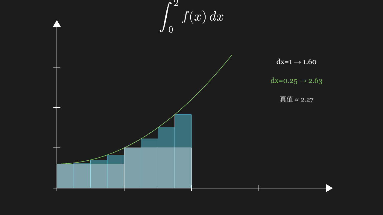
"""黎曼和逼近积分

@expect 矩形越分越细、矩形面积之和越来越接近定积分值:粗分 dx=1 的矩形以描边 ghost 留在终态
        与细分 dx=0.25 对照,右侧两行标注给出两档的面积和(1.60 → 2.63,真值 2.27)。
@template 要讲「细分 / 求和逼近」(黎曼和、梯形近似、级数部分和这类越分越准的画面)时照它抄。
@note 讲解模板:同一段区间把 dx 变小,矩形和逼近曲线下的面积;
    粗分矩形在 Transform 前 copy 存档,变换后以低透明度描边 add 回去,才有「从什么变到什么」的对照
"""

from manim import *


class RiemannSumScene(Scene):
    def construct(self):
        ax = Axes(x_range=[0, 4, 1], y_range=[0, 4, 1])
        # 曲线只画到 x=2.6:0.4*2.6²+0.6≈3.3,峰落在 y_range=[0,4] 内不被上缘裁断
        graph = ax.plot(lambda x: 0.4 * x * x + 0.6, x_range=[0, 2.6], color=GREEN)
        coarse = ax.get_riemann_rectangles(graph, x_range=[0, 2], dx=1)
        fine = ax.get_riemann_rectangles(graph, x_range=[0, 2], dx=0.25)
        formula = MathTex(r"\int_0^2 f(x)\,dx").move_to([0, 3.4, 0])

        # 粗分存档:Transform 前抄一份,终态以低透明度描边留在原位对照
        coarse_ghost = coarse.copy().set_fill(opacity=0).set_stroke(WHITE, width=1.5, opacity=0.7)

        note_coarse = Text("dx=1 → 1.60", font_size=26, color=WHITE).move_to([3.9, 1.7, 0])
        note_fine = Text("dx=0.25 → 2.63", font_size=26, color=GREEN).move_to([3.9, 1.0, 0])
        note_true = Text("真值 ≈ 2.27", font_size=24, color=GRAY_A).move_to([3.9, 0.3, 0])

        self.play(Create(ax), Create(graph))
        self.play(Write(formula), FadeIn(coarse))
        self.play(Transform(coarse, fine))
        self.add(coarse_ghost)
        self.play(Write(note_coarse), Write(note_fine), Write(note_true), run_time=0.8)
        self.wait(0.3)
Linear map: rotation
Grid and vectors rotate 30° as a whole (not a multiple of 90°, so the tilted orientation is obvious) without changing shape; the matrix is written in cos/sin 30° form, the green arrow is 2 cells long and still aligns with the grid ticks after rotation.
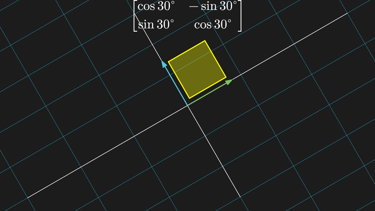
"""线性变换:旋转

@expect 网格与向量整体旋转 30°(非 90° 倍数,网格斜过来朝向明显变了),形状不变;
        矩阵写成 cos/sin 30° 的形式,绿色箭头长 2 格、旋转后仍对齐网格刻度。
@note 讲解模板:ApplyMatrix 把基向量与图形一起按矩阵搬过去;
    旋转角避开 90° 的倍数——90° 时网格与原来重合,看不出转没转
"""

from manim import *
import math


class RotationTransformScene(Scene):
    def construct(self):
        c, s = math.cos(math.radians(30)), math.sin(math.radians(30))
        # 网格与向量一起参与变换,让「整体旋转」看得见
        plane = NumberPlane(
            x_range=[-3, 3, 1],
            y_range=[-3, 3, 1],
            background_line_style={"stroke_color": BLUE_D, "stroke_width": 1.5},
            axis_config={"stroke_color": GRAY_D},
        )
        basis = VGroup(
            Arrow(start=ORIGIN, end=RIGHT * 2, color=GREEN),
            Arrow(start=ORIGIN, end=UP * 2, color=BLUE),
        )
        square = Square(side_length=1.6, color=YELLOW)
        square.set_fill(YELLOW, 0.35)
        square.move_to(RIGHT + UP)
        figure = VGroup(plane, basis, square)
        title = MathTex(
            r"\begin{bmatrix} \cos 30^\circ & -\sin 30^\circ \\ \sin 30^\circ & \cos 30^\circ \end{bmatrix}"
        ).move_to([0, 3.4, 0])

        self.play(Create(figure), Write(title))
        self.play(ApplyMatrix([[c, -s], [s, c]], figure), run_time=2)
        self.wait(0.3)
Linear map: shear
The grid is sheared: rows shift horizontally and columns tilt; the pre-image grid stays in place as a low-opacity ghost for comparison, and a 1×1 reference square becomes a parallelogram with the same base and height — area per cell unchanged (det=1), visibly.
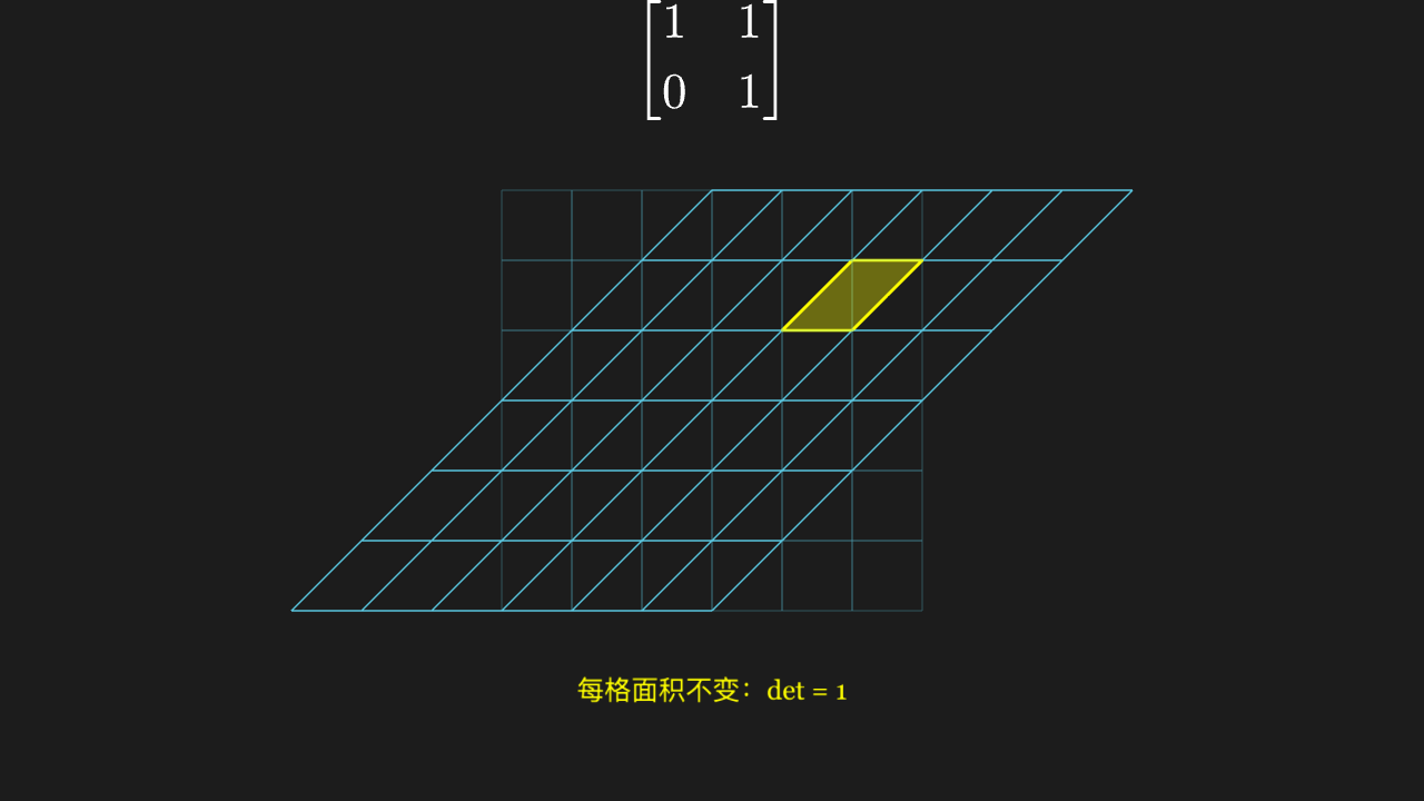
"""线性变换:剪切

@expect 网格被剪切:横行水平错动、竖列倾斜,变换前网格以低透明度 ghost 留在原位对照,
        一个 1×1 参照正方形变成同底同高的平行四边形——「每格面积不变(det=1)」看得见。
@note 讲解模板:剪切矩阵把竖直方向推向水平方向,网格最能看出来;
    ghost(copy 低透明度、不参与 ApplyMatrix)给出「原来是什么」的对照
"""

from manim import *


class ShearTransformScene(Scene):
    def construct(self):
        cells = VGroup()
        for i in range(-3, 3):
            for j in range(-3, 3):
                cell = Square(side_length=0.7, color=BLUE, stroke_width=1.5)
                cell.move_to([i * 0.7 + 0.35, j * 0.7 + 0.35, 0])
                cells.add(cell)

        # 变换前 ghost:低透明度网格留原位,不参与变换
        ghost = cells.copy().set_stroke(GREY, width=1, opacity=0.35)

        # 1×1 参照正方形:剪切后底和高都不变,只是被推歪
        unit = Square(side_length=0.7, color=YELLOW, stroke_width=3).set_fill(YELLOW, 0.35)
        unit.move_to([-0.35 + 0.7, 0.35 + 0.7, 0])

        title = MathTex(r"\begin{bmatrix} 1 & 1 \\ 0 & 1 \end{bmatrix}").move_to([0, 3.4, 0])
        note = Text("每格面积不变:det = 1", font_size=26, color=YELLOW).move_to([0, -2.9, 0])

        self.play(Create(ghost), Create(cells), Write(title))
        self.play(FadeIn(unit), run_time=0.5)
        self.play(ApplyMatrix([[1, 1], [0, 1]], VGroup(cells, unit)), run_time=2)
        self.play(Write(note), run_time=0.5)
        self.wait(0.3)
Linear map: eigen directions
Vectors on an eigen direction stay on that direction after the map (red v₁ stretched 3× along the dashed line, blue v₂ unmoved) while the grey control vector u leaves its direction — deflected and undeflected side by side; the dashed lines are the two eigen directions. The three pre-image vectors stay in place as translucent ghosts, with λ₁=3 / λ₂=1 labels near the arrow tips.
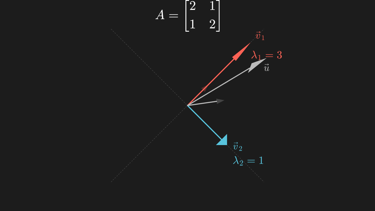
"""线性变换:特征方向

@expect 特征方向上的向量变换后仍在这条方向上(红 v₁ 沿虚线拉长 3 倍、蓝 v₂ 不动),
灰色对照向量 u 变换后偏离原方向——偏折的与不偏折的对照着看;虚线即两条特征方向。
变换前三根向量以半透明 ghost 留原位,箭头尖附近有 λ₁=3 / λ₂=1 标注。
@template 要讲线性变换 / 矩阵作用于图形与向量(网格变形、变换前后对照、找不变方向)时照它抄。
@note 讲解模板:变换后方向不变的向量就是特征向量(A 的特征值 3 与 1,特征方向 [1,1] 与 [1,-1])
"""

from manim import *
import numpy as np


class EigenvectorScene(Scene):
    def construct(self):
        A = np.array([[2.0, 1.0], [1.0, 2.0]])

        # 两条特征方向虚线([1,1] 与 [1,-1])
        dash_e1 = DashedLine([-2.9, -2.9, 0], [2.9, 2.9, 0], color=GRAY_D, stroke_width=1.5)
        dash_e2 = DashedLine([-2.9, 2.9, 0], [2.9, -2.9, 0], color=GRAY_D, stroke_width=1.5)

        # 特征向量缩短初始长度,拉长 3 倍后仍不出框
        vec_a = Arrow(start=ORIGIN, end=[0.8, 0.8, 0], color=RED, buff=0)
        vec_b = Arrow(start=ORIGIN, end=[1.5, -1.5, 0], color=BLUE, buff=0)
        # 非特征对照向量,变换后明显偏折([1,1] 方向的 v₁ 不偏,对照才醒目)
        vec_c = Arrow(start=ORIGIN, end=[1.4, 0.2, 0], color=GRAY_B, buff=0)

        t = ValueTracker(0)

        def tip(v):
            """从初始端点插值到 A·v 的端点,供标签跟随(不用 MathTex 包围盒定位)"""
            v = np.asarray(v, dtype=float)
            w = A @ v[:2]
            return (1 - t.get_value()) * v + t.get_value() * np.array([w[0], w[1], 0.0])

        label_a = MathTex(r"\vec v_1", color=RED, font_size=36)
        label_a.add_updater(lambda m: m.move_to(tip([0.8, 0.8, 0]) + UP * 0.25 + RIGHT * 0.35))
        label_b = MathTex(r"\vec v_2", color=BLUE, font_size=36)
        label_b.add_updater(lambda m: m.move_to(tip([1.5, -1.5, 0]) + DOWN * 0.05 + RIGHT * 0.4))
        label_c = MathTex(r"\vec u", color=GRAY_B, font_size=36)
        label_c.add_updater(lambda m: m.move_to(tip([1.4, 0.2, 0]) + DOWN * 0.35))

        title = MathTex(r"A = \begin{bmatrix} 2 & 1 \\ 1 & 2 \end{bmatrix}").move_to([0, 3.4, 0])

        self.play(FadeIn(dash_e1), FadeIn(dash_e2))
        self.play(Create(vec_a), Create(vec_b), Create(vec_c), Write(title))
        self.play(Write(label_a), Write(label_b), Write(label_c), run_time=0.6)

        # 变换前 ghost:三根向量以低透明度留原位(不参与变换),供 before/after 对照
        ghosts = VGroup(vec_a.copy(), vec_b.copy(), vec_c.copy()).set_opacity(0.25)
        self.play(FadeIn(ghosts), run_time=0.5)

        self.play(
            ApplyMatrix([[2, 1], [1, 2]], VGroup(vec_a, vec_b, vec_c)),
            t.animate.set_value(1),
            run_time=2,
        )
        # 特征值标注:单个 MathTex 直接 move_to 到对应箭头尖附近
        lam_1 = MathTex(r"\lambda_1=3", color=RED, font_size=40).move_to([3.0, 1.9, 0])
        lam_2 = MathTex(r"\lambda_2=1", color=BLUE, font_size=40).move_to([2.3, -2.1, 0])
        self.play(Write(lam_1), Write(lam_2), run_time=0.7)
        self.wait(0.3)
Probability: frequency of dice rolls
The more rolls, the flatter the six frequency bars become (approaching uniform): six nearly equal bars (15%–18%), each measured value hovering around the orange dashed line at the theoretical 16.7%.
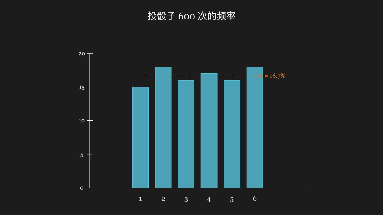
"""概率:投骰子的频率

@expect 掷骰子次数越多,六面的频率柱越来越齐平(趋近均匀):六根柱几乎等高(15%–18%),
实测值都贴着理论值 16.7% 的橙色虚线附近起伏。
@template 要画「随机模拟 + 频率柱状图 + 理论值对照线」(大数定律、蒙特卡洛这类实验对照理论)时照它抄。
@note 讲解模板:BarChart 画实测频率,与理论值 1/6 对照;BarChart 默认摆位偏右上、
      上缘刻度会被裁,需整体 move_to 居中偏下并收紧 y_range;刻度用整数百分比
      (适配层把两位小数刻度标签四舍五入到一位,0.05 步进会显示成重复的 0.2/0.1);
      BarChart 实例不挂 c2p(只有 Axes 桥接),参考线按图表几何手算绝对坐标
"""

from manim import *


class DiceFrequencyScene(Scene):
    def construct(self):
        observed_pct = [15, 18, 16, 17, 16, 18]
        chart = BarChart(
            values=observed_pct,
            y_range=[0, 20, 5],
            bar_colors=[BLUE],
        )
        chart.move_to([0, -0.7, 0])
        title = Text("投骰子 600 次的频率", font_size=34).move_to([0, 3.4, 0])

        # 理论值 1/6=16.7% 的参考线:量程 20 对应轴高 5 单位(默认 y_length),
        # 16.7% 高度 = 16.7/20*5 ≈ 4.2;轴底经实测标定在 y≈-3.0
        guide = DashedLine(
            [-1.9, -3.0 + 16.7 / 20 * 5, 0],
            [1.9, -3.0 + 16.7 / 20 * 5, 0],
            color=ORANGE,
            stroke_width=2.5,
        )
        guide_label = Text("1/6 ≈ 16.7%", font_size=22, color=ORANGE)
        guide_label.move_to([2.9, -3.0 + 16.7 / 20 * 5, 0])

        self.play(Write(title))
        self.play(Create(chart))
        self.play(Create(guide), Write(guide_label))
        self.wait(0.3)
Probability: binomial distribution
Two binomial pmf polylines side by side: n=10 peaks near 0.25 and n=30 near 0.14 — same p, larger n gives a shorter and wider distribution; the two-way comparison carries the claim that the parameters decide the shape.
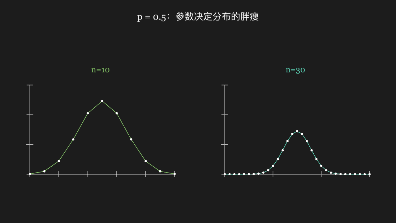
"""概率:二项分布

@expect 两组二项分布 pmf 折线并排:n=10 峰值约 0.25、n=30 峰值约 0.14——
        同样的 p,n 越大分布越矮越宽,「参数决定胖瘦」靠两组对照成立。
@note 讲解模板:n 次试验成功 k 次的概率——p 相同、n 不同,两组折线对照着看;
      BarChart 默认摆位偏右上且宽度不受 x_length 约束、两组会重叠出框,
      降级用 Axes.plot_line_graph 左右各占半幅;
      "p = 0.5" 里的 p 斜体字形易缺字,标题一律用 Text 不用 MathTex
"""

from manim import *
import math


class BinomialScene(Scene):
    def construct(self):
        ks_10 = list(range(11))
        pmf_10 = [math.comb(10, k) * 0.5 ** 10 for k in ks_10]
        ks_30 = list(range(31))
        pmf_30 = [math.comb(30, k) * 0.5 ** 30 for k in ks_30]

        ax_10 = Axes(
            x_range=[0, 10, 2],
            y_range=[0, 0.3, 0.1],
            x_length=5.2,
            y_length=3.2,
            tips=False,
            axis_config={"color": GRAY_B},
        )
        ax_10.move_to([-3.5, -0.7, 0])
        graph_10 = ax_10.plot_line_graph(ks_10, pmf_10, add_vertex_dots=True,
                                         line_color=GREEN, vertex_dot_radius=0.04)

        ax_30 = Axes(
            x_range=[0, 30, 10],
            y_range=[0, 0.3, 0.1],
            x_length=5.2,
            y_length=3.2,
            tips=False,
            axis_config={"color": GRAY_B},
        )
        ax_30.move_to([3.5, -0.7, 0])
        graph_30 = ax_30.plot_line_graph(ks_30, pmf_30, add_vertex_dots=True,
                                         line_color=TEAL, vertex_dot_radius=0.04)

        label_10 = Text("n=10", font_size=28, color=GREEN).move_to([-3.5, 1.5, 0])
        label_30 = Text("n=30", font_size=28, color=TEAL).move_to([3.5, 1.5, 0])
        title = Text("p = 0.5:参数决定分布的胖瘦", font_size=32).move_to([0, 3.4, 0])

        self.play(Write(title))
        self.play(Create(ax_10), Create(graph_10), Write(label_10), run_time=1.2)
        self.play(Create(ax_30), Create(graph_30), Write(label_30), run_time=1.2)
        self.wait(0.3)
Spatial Cartesian coordinates and a cube
A cube of edge 2 seen at an angle: three faces visible at once with different shading (lit and with depth, not a black blob); it sits in the first octant with a yellow dot and label on its farthest vertex (2, 2, 2); the three axes leave the origin with Z pointing up. The title is pinned to the top-left of the frame and does not follow the camera. The camera first spins about its azimuth and then animates to the other side — the final frame shows a different set of side faces than the initial view, proving the camera really moved instead of a 2D-flattened face.
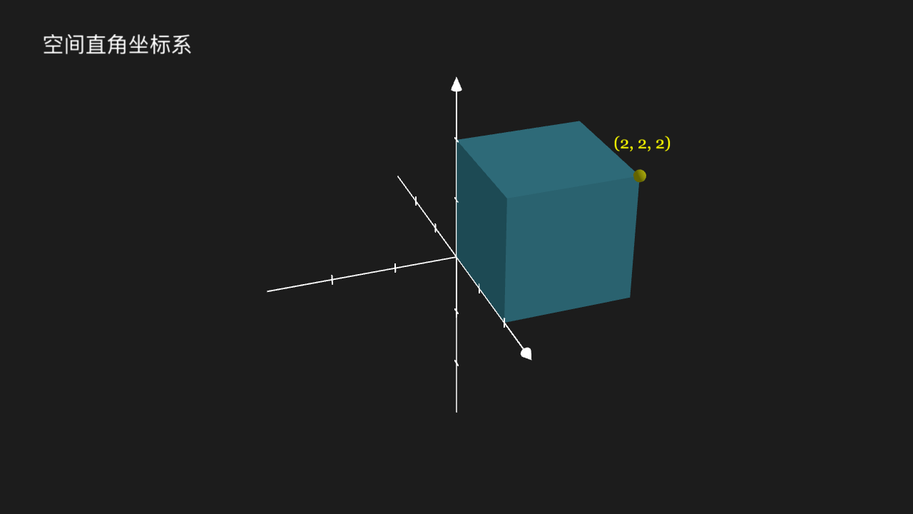
"""空间直角坐标系与立方体

@expect 斜视看一个棱长 2 的立方体:三个面同时可见、明暗各不同(有光有深度,不是一块黑);
        它坐在第一象限,最远的顶点 (2, 2, 2) 上有个黄点、旁边跟着黄色标注;
        三条坐标轴从原点穿出,Z 轴朝上。标题钉在画面左上角、不跟相机跑。
        相机先绕方位角自转一段,再动画转到另一侧——终帧看到的是立方体的另一组侧面,
        与初始斜视完全不同,证明相机真动了,不是被 2D 拍扁的一张脸。
@template 要画 3D 空间图形(立方体 / 球 / 多面体 / 坐标轴)或想让相机转起来时照它抄。
@note 3D 物体**必须**写 class X(ThreeDScene):普通的 Scene 里一盏灯都没有,
      吃光的材质落进去就是一团纯黑(不是「3D 没实现」,是放错场景了)。
      屏幕上的字用 add_fixed_in_frame_mobjects 钉住;3D 里跟着物体走、又要一直正对镜头的字
      用 add_fixed_orientation_mobjects——斜视下它俩都不会被压扁。
      3D 实体的颜色 / 透明用构造参数 color / opacity(CE 的 fill_color / fill_opacity 在 3D 实体上不生效)。
"""

from manim import *

SIDE = 2.0


class SpaceCubeScene(ThreeDScene):
    def construct(self):
        # 轴比默认短一圈(默认 x∈[-6,6]、z∈[-4,4],斜视下会顶到画面边):
        # 立方体已经占住画面中心,轴只用来交代「这是个坐标系」。
        axes = ThreeDAxes(x_range=[-3, 3, 1], y_range=[-3, 3, 1], z_range=[-3, 3, 1])
        cube = Cube(side_length=SIDE, color=BLUE)
        cube.shift([SIDE / 2, SIDE / 2, SIDE / 2])  # 坐进第一象限,别跟坐标轴原点叠在一起
        corner = Dot3D(point=[SIDE, SIDE, SIDE], radius=0.09, color=YELLOW)

        title = Text("空间直角坐标系", font_size=32)
        title.to_corner(UL)
        self.add_fixed_in_frame_mobjects(title)  # 钉在屏幕上:不跟相机转,也不会被斜视压扁

        corner_label = Text("(2, 2, 2)", font_size=22, color=YELLOW)
        corner_label.move_to([SIDE, SIDE, SIDE + 0.5])
        self.add_fixed_orientation_mobjects(corner_label)  # 留在 3D 里,但永远正对镜头

        self.set_camera_orientation(phi=70 * DEGREES, theta=-135 * DEGREES)  # 初始斜视
        self.play(Create(axes), FadeIn(cube), FadeIn(corner), Write(title), run_time=1)
        self.begin_ambient_camera_rotation(rate=0.4)  # 相机自己绕方位角慢慢转
        self.wait(1.5)
        self.stop_ambient_camera_rotation()
        self.move_camera(phi=60 * DEGREES, theta=-20 * DEGREES, run_time=2)  # 再动画转到另一侧
        self.wait(0.2)