概率论与统计
容斥、条件概率、贝叶斯树、期望与方差、大数定律、中心极限、泊松、3σ 法则、蒙特卡洛 π、随机游走与假设检验。
本页 12 条示例。代码引自 corpus/examples/math-prob/,截图为真机渲染的终态。
概率的加法公式(容斥):P(A∪B) = P(A) + P(B) - P(A∩B)
样本空间 Ω 里两个半透明矩形事件 A、B 相互交叠,重叠区由两层填色混出中间色;A∩B 用红色描边框单独点亮并标注字母,再回到公式里说明它刚好是被重复计入的那一份。
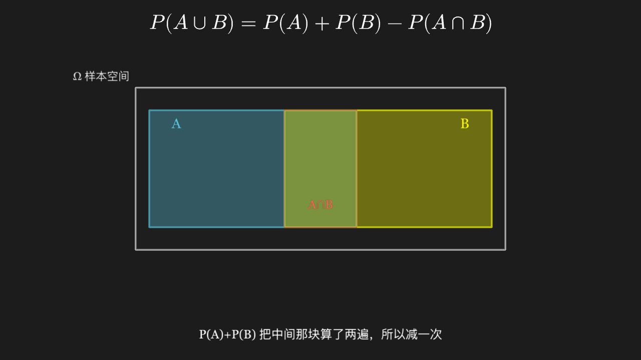
"""概率的加法公式(容斥):P(A∪B) = P(A) + P(B) - P(A∩B)

@expect 样本空间 Ω 里两个半透明矩形事件 A、B 相互交叠,重叠区由两层填色混出中间色;A∩B 用红色描边框单独点亮并标注字母,再回到公式里说明它刚好是被重复计入的那一份。
@note 讲解要点:容斥公式的「减一次交集」不是凑出来的修正项——P(A)+P(B) 把 A∩B 里的概率计了两遍,减掉它才算不重不漏。
"""

from manim import *


class InclusionExclusionScene(Scene):
    def construct(self):
        space = Rectangle(width=8.2, height=3.6, color=GRAY_B).move_to([0, 0.25, 0])
        space.set_fill(GRAY_E, opacity=0.35)

        a_box = Rectangle(width=4.6, height=2.6, color=BLUE).move_to([-1.5, 0.25, 0])
        b_box = Rectangle(width=4.6, height=2.6, color=YELLOW).move_to([1.5, 0.25, 0])
        inter = Rectangle(width=1.6, height=2.6, color=RED).move_to([0, 0.25, 0])
        a_box.set_fill(BLUE, opacity=0.35)
        b_box.set_fill(YELLOW, opacity=0.35)
        inter = Rectangle(width=1.6, height=2.6, color=RED, stroke_width=3).move_to([0, 0.25, 0])

        label_omega = Text("Ω 样本空间", font_size=24, color=GRAY_A).next_to(space, UL, buff=0.14)
        label_a = Text("A", font_size=30, color=BLUE).move_to([-3.2, 1.25, 0])
        label_b = Text("B", font_size=30, color=YELLOW).move_to([3.2, 1.25, 0])
        label_inter = Text("A∩B", font_size=26, color=RED).move_to([0, -0.55, 0])

        formula = MathTex(r"P(A\cup B) = P(A) + P(B) - P(A\cap B)", font_size=44).to_edge(UP, buff=0.3)
        caption = Text(
            "P(A)+P(B) 把中间那块算了两遍,所以减一次",
            font_size=26,
        ).to_edge(DOWN, buff=0.4)

        self.play(Create(space), Write(label_omega), run_time=0.8)
        self.play(Write(formula), run_time=0.8)
        self.play(Create(a_box), Create(b_box), Write(label_a), Write(label_b), run_time=1.0)
        self.play(Create(inter), Write(label_inter), run_time=0.6)
        self.play(Circumscribe(inter, color=WHITE, stroke_width=3), run_time=0.9)
        self.play(Write(caption), run_time=0.7)
        self.wait(0.4)
条件概率:换一个样本空间重新归一化
事件 A 被 B 的边界切成两半,先点亮落在 B 里的那一半;随后 B 之外的部分整体压暗,只剩 B 内部重新按比例摊开。
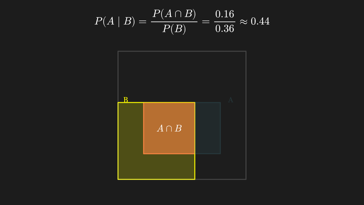
"""条件概率:换一个样本空间重新归一化

@expect 事件 A 被 B 的边界切成两半,先点亮落在 B 里的那一半;随后 B 之外的部分整体压暗,只剩 B 内部重新按比例摊开。
@note 讲解要点:P(A|B) 的分母从 Ω 换成了 B——不是给 A 打折扣,而是「已知 B 发生」之后把概率全部压回 B 内部重新分配。
"""

from manim import *


class ConditionalProbabilityScene(Scene):
    def construct(self):
        omega = Rectangle(width=5.0, height=5.0, color=GRAY_B).move_to([0, -0.5, 0])
        omega.set_fill(GRAY_E, opacity=0.3)

        b_box = Rectangle(width=3.0, height=3.0, color=YELLOW).move_to([-1.0, -1.5, 0])
        b_box.set_fill(YELLOW, opacity=0.22)

        a_inside = Rectangle(width=2.0, height=2.0, color=RED).move_to([-0.5, -1.0, 0])
        a_outside = Rectangle(width=1.0, height=2.0, color=BLUE).move_to([1.0, -1.0, 0])
        a_inside.set_fill(RED, opacity=0.6)
        a_outside.set_fill(BLUE, opacity=0.6)

        label_a = Text("A", font_size=28, color=BLUE).move_to([1.9, 0.1, 0])
        label_b = Text("B", font_size=28, color=YELLOW).move_to([-2.2, 0.1, 0])
        label_ab = MathTex(r"A\cap B", font_size=36, color=WHITE).move_to([-0.5, -1.0, 0])

        formula = MathTex(
            r"P(A\mid B) = \frac{P(A\cap B)}{P(B)} = \frac{0.16}{0.36} \approx 0.44",
            font_size=40,
        ).to_edge(UP, buff=0.35)

        self.play(Create(omega), run_time=0.6)
        self.play(Write(formula), run_time=0.8)
        self.play(Create(a_outside), Create(a_inside), Write(label_a), run_time=0.8)
        self.play(Create(b_box), Write(label_b), run_time=0.7)
        self.play(Write(label_ab), Indicate(a_inside, color=WHITE, scale_factor=1.05), run_time=0.8)
        self.play(
            a_outside.animate.set_opacity(0.12),
            a_inside.animate.set_opacity(1.0),
            omega.animate.set_opacity(0.25),
            b_box.animate.set_opacity(1.0),
            label_a.animate.set_opacity(0.15),
            run_time=1.0,
        )
        self.wait(0.4)
贝叶斯公式:一棵树上把先验和似然合成后验
左侧两层分叉的树把「患病 1% × 检出 99%」和「健康 99% × 误报 5%」两条路分别铺开;右侧列出两条路的联合概率,绿色那条阳性总概率是分母,红色那条占比就是后验。
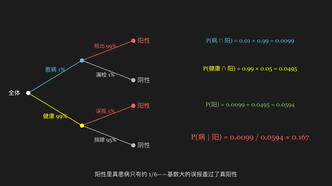
"""贝叶斯公式:一棵树上把先验和似然合成后验

@expect 左侧两层分叉的树把「患病 1% × 检出 99%」和「健康 99% × 误报 5%」两条路分别铺开;右侧列出两条路的联合概率,绿色那条阳性总概率是分母,红色那条占比就是后验。
@note 讲解要点:阳性结果里真患病只占约 1/6——因为健康人基数大,哪怕误报率只有 5%,误报的绝对数量也远大于真阳性。这就是「基率」被忽略的代价。
"""

from manim import *

ROOT = [-5.9, 0, 0]
LV2_SICK = [-3.6, 1.4, 0]
LV2_WELL = [-3.6, -1.4, 0]
LV3_POS_SICK = [-1.4, 2.25, 0]
LV3_NEG_SICK = [-1.4, 0.55, 0]
LV3_POS_WELL = [-1.4, -0.55, 0]
LV3_NEG_WELL = [-1.4, -2.25, 0]


class BayesTreeScene(Scene):
    def construct(self):
        branch = lambda a, b, c=GRAY_B: Line(a, b, color=c, stroke_width=2.5)

        trunk = VGroup(branch(ROOT, LV2_SICK, BLUE), branch(ROOT, LV2_WELL, YELLOW))
        upper = VGroup(branch(LV2_SICK, LV3_POS_SICK, RED), branch(LV2_SICK, LV3_NEG_SICK))
        lower = VGroup(branch(LV2_WELL, LV3_POS_WELL, RED), branch(LV2_WELL, LV3_NEG_WELL))

        root_dot = Dot(ROOT, radius=0.09, color=WHITE)
        level2_dots = VGroup(
            Dot(LV2_SICK, radius=0.09, color=BLUE),
            Dot(LV2_WELL, radius=0.09, color=YELLOW),
        )
        leaves = VGroup(
            Dot(LV3_POS_SICK, radius=0.09, color=RED),
            Dot(LV3_NEG_SICK, radius=0.09, color=GRAY_B),
            Dot(LV3_POS_WELL, radius=0.09, color=RED),
            Dot(LV3_NEG_WELL, radius=0.09, color=GRAY_B),
        )

        head_labels = VGroup(
            Text("全体", font_size=24).move_to([-6.5, 0, 0]),
            Text("患病 1%", font_size=24, color=BLUE).move_to([-4.75, 1.0, 0]),
            Text("健康 99%", font_size=24, color=YELLOW).move_to([-4.75, -1.0, 0]),
        )
        rate_labels = VGroup(
            Text("检出 99%", font_size=22, color=RED).move_to([-2.6, 2.02, 0]),
            Text("漏检 1%", font_size=22, color=GRAY_A).move_to([-2.6, 0.78, 0]),
            Text("误报 5%", font_size=22, color=RED).move_to([-2.6, -0.78, 0]),
            Text("排除 95%", font_size=22, color=GRAY_A).move_to([-2.6, -2.02, 0]),
        )
        leaf_labels = VGroup(
            Text("阳性", font_size=26, color=RED).move_to([-0.95, 2.25, 0]),
            Text("阴性", font_size=26, color=GRAY_B).move_to([-0.95, 0.55, 0]),
            Text("阳性", font_size=26, color=RED).move_to([-0.95, -0.55, 0]),
            Text("阴性", font_size=26, color=GRAY_B).move_to([-0.95, -2.25, 0]),
        )

        line_sick_pos = Text("P(病 ∩ 阳) = 0.01 × 0.99 = 0.0099", font_size=24, color=BLUE)
        line_sick_pos.move_to([3.6, 2.25, 0])
        line_well_pos = Text("P(健康 ∩ 阳) = 0.99 × 0.05 = 0.0495", font_size=24, color=YELLOW)
        line_well_pos.move_to([3.6, 1.05, 0])
        line_total = Text("P(阳) = 0.0099 + 0.0495 = 0.0594", font_size=24, color=GREEN)
        line_total.move_to([3.6, -0.5, 0])
        posterior = Text("P(病 | 阳) = 0.0099 / 0.0594 ≈ 0.167", font_size=30, color=RED)
        posterior.move_to([3.6, -1.9, 0])

        caption = Text("阳性里真患病只有约 1/6——基数大的误报盖过了真阳性", font_size=24, color=GRAY_A)
        caption.to_edge(DOWN, buff=0.35)

        self.play(Create(trunk), FadeIn(root_dot), run_time=0.8)
        self.play(Write(head_labels), FadeIn(level2_dots), run_time=0.8)
        self.play(Create(upper), Create(lower), FadeIn(leaves), run_time=1.0)
        self.play(Write(rate_labels), run_time=0.9)
        self.play(Write(leaf_labels), run_time=0.8)
        self.play(Write(line_sick_pos), Write(line_well_pos), run_time=0.9)
        self.play(Write(line_total), run_time=0.7)
        self.play(Write(posterior), run_time=0.9)
        self.play(Write(caption), run_time=0.8)
        self.wait(0.4)
期望:概率分布的「重心」,也是这根杠杆的支点
六个取值位置上立着高度正比于概率的方块,杠杆在正中间找到平衡——支点恰好落在加权平均 μ=3.6 处,而不是算术中心 3.5。
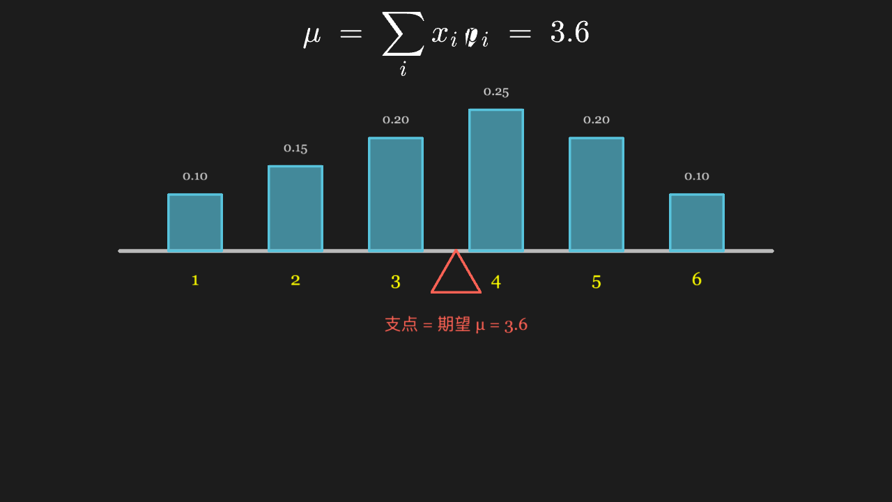
"""期望:概率分布的「重心」,也是这根杠杆的支点

@expect 六个取值位置上立着高度正比于概率的方块,杠杆在正中间找到平衡——支点恰好落在加权平均 μ=3.6 处,而不是算术中心 3.5。
@note 讲解要点:期望就是「按概率加权后的平均位置」。概率大的取值把支点拉向自己,和物理杠杆完全同构——这也是期望才叫「均值」的原因。
"""

from manim import *


class ExpectationBalanceScene(Scene):
    def construct(self):
        faces = [1, 2, 3, 4, 5, 6]
        weights = [0.10, 0.15, 0.20, 0.25, 0.20, 0.10]
        mean = sum(f * w for f, w in zip(faces, weights))

        x_at = lambda face: -4.0 + (face - 1) * 1.6
        beam = Line([-5.2, 0, 0], [5.2, 0, 0], color=GRAY_B, stroke_width=6)

        blocks = VGroup()
        for face, w in zip(faces, weights):
            block = Rectangle(width=0.85, height=w * 9.0, color=BLUE)
            block.set_fill(BLUE, opacity=0.65)
            block.move_to([x_at(face), w * 9.0 / 2, 0])
            blocks.add(block)

        face_labels = VGroup()
        for face in faces:
            face_labels.add(
                Text(str(face), font_size=28, color=YELLOW).move_to([x_at(face), -0.45, 0])
            )

        weight_labels = VGroup()
        for face, w in zip(faces, weights):
            weight_labels.add(
                Text(f"{w:.2f}", font_size=20, color=GRAY_A).move_to([x_at(face), w * 9.0 + 0.3, 0])
            )

        pivot_x = x_at(mean)
        fulcrum = Triangle(color=RED).scale(0.45).move_to([pivot_x, -0.32, 0])
        pivot_label = Text("支点 = 期望 μ = 3.6", font_size=26, color=RED)
        pivot_label.next_to(fulcrum, DOWN, buff=0.35)

        # MathTex 定位用绝对坐标:to_edge 要读包围盒,包围盒由 KaTeX 异步量出,量出前是 NaN(时隐时现)
        formula = MathTex(r"\mu \;=\; \sum_i x_i\, p_i \;=\; 3.6", font_size=48).move_to([0, 3.3, 0])

        self.play(Write(formula), run_time=1.0)
        self.play(Create(beam), run_time=0.5)
        self.play(LaggedStart(*[FadeIn(b) for b in blocks], lag_ratio=0.1), run_time=1.4)
        self.play(Write(face_labels), Write(weight_labels), run_time=0.8)
        self.play(FadeIn(fulcrum), Write(pivot_label), run_time=0.8)
        self.play(Indicate(blocks[3], color=RED, scale_factor=1.06), run_time=0.6)
        self.wait(0.4)
方差刻画离散程度:同期望,不同「撒得开」
上下一共两组数据共享同一条数轴和同一个均值刻度,但一组的点挤成一撮、另一组散得很开;两条两端带短竖线端点标记的横线标出各自的极差,视觉差距直接对应方差 2 与 200。
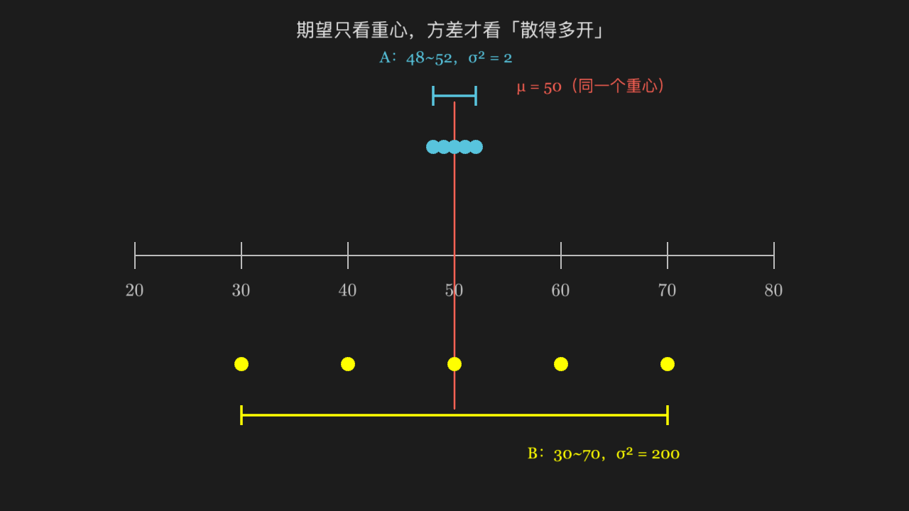
"""方差刻画离散程度:同期望,不同「撒得开」

@expect 上下一共两组数据共享同一条数轴和同一个均值刻度,但一组的点挤成一撮、另一组散得很开;两条两端带短竖线端点标记的横线标出各自的极差,视觉差距直接对应方差 2 与 200。
@note 讲解要点:均值只告诉你「重心在哪」,完全说不出「有多散」——两组数据 μ 都是 50,却是完全不同的两个分布。方差就是把这个「散」量化出来的量。
"""

from manim import *


class VarianceSpreadScene(Scene):
    def construct(self):
        group_a = [48, 49, 50, 51, 52]
        group_b = [30, 40, 50, 60, 70]
        x_of = lambda v: -5.0 + (v - 20) / 6.0

        axis = NumberLine(
            x_range=[20, 80, 10],
            length=10.0,
            include_numbers=True,
            color=GRAY_B,
        )
        mean_line = Line([0, -2.4, 0], [0, 2.4, 0], color=RED, stroke_width=3)

        dots_a = VGroup(*[Dot([x_of(v), 1.7, 0], radius=0.11, color=BLUE) for v in group_a])
        dots_b = VGroup(*[Dot([x_of(v), -1.7, 0], radius=0.11, color=YELLOW) for v in group_b])

        def span_line(x1, x2, y, color):
            bar = Line([x1, y, 0], [x2, y, 0], color=color, stroke_width=4)
            cap_l = Line([x1, y - 0.14, 0], [x1, y + 0.14, 0], color=color, stroke_width=4)
            cap_r = Line([x2, y - 0.14, 0], [x2, y + 0.14, 0], color=color, stroke_width=4)
            return VGroup(bar, cap_l, cap_r)

        span_a = span_line(x_of(48), x_of(52), 2.5, BLUE)
        span_b = span_line(x_of(30), x_of(70), -2.5, YELLOW)

        txt = lambda s, c=WHITE, fs=26: Text(s, font_size=fs, color=c)
        labels = VGroup(
            txt("μ = 50(同一个重心)", RED, 24).next_to(mean_line, UP, buff=0.1).shift(RIGHT * 2.2),
            txt("A:48~52,σ² = 2", BLUE, 24).move_to([x_of(48) + 0.2, 3.1, 0]),
            txt("B:30~70,σ² = 200", YELLOW, 24).move_to([x_of(70) - 1.0, -3.1, 0]),
        )

        title = txt("期望只看重心,方差才看「散得多开」", GRAY_A, 28).to_edge(UP, buff=0.3)

        self.play(Write(title), run_time=0.7)
        self.play(Create(axis), run_time=0.7)
        self.play(FadeIn(dots_a), Create(span_a), Write(labels[1]), run_time=1.0)
        self.play(Create(mean_line), Write(labels[0]), run_time=0.8)
        self.play(FadeIn(dots_b), Create(span_b), Write(labels[2]), run_time=1.0)
        self.wait(0.4)
大数定律:频率随试验次数增加而贴向真实概率
一条从剧烈上下抖动开始、越往右摆幅越小的折线,逐渐收拢到 y=0.5 那条理论概率的虚线上——收敛是「以概率 1」的,不是每一步都单调靠近。
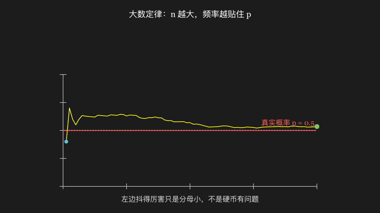
"""大数定律:频率随试验次数增加而贴向真实概率

@expect 一条从剧烈上下抖动开始、越往右摆幅越小的折线,逐渐收拢到 y=0.5 那条理论概率的虚线上——收敛是「以概率 1」的,不是每一步都单调靠近。
@note 讲解要点:折线在左侧跳得厉害并不代表不公平;大数定律说的是 n 趋于无穷时频率依概率收敛到 p。前几步的偏差会被庞大的分母稀释掉。
"""

from manim import *
import numpy as np


class LawOfLargeNumbersScene(Scene):
    def construct(self):
        rng = np.random.default_rng(2024)
        n_max = 400
        flips = (rng.random(n_max) < 0.5).astype(float)
        freq = np.cumsum(flips) / np.arange(1, n_max + 1)

        ax = Axes(
            x_range=[0, 400, 100],
            y_range=[0, 1, 0.25],
            x_length=9.5,
            y_length=4.2,
            tips=False,
            axis_config={"color": GRAY_B},
        )
        ax.shift(DOWN * 0.9)

        true_line = DashedLine(ax.c2p(0, 0.5), ax.c2p(400, 0.5), color=RED)
        true_label = Text("真实概率 p = 0.5", font_size=26, color=RED)
        true_label.next_to(true_line, UP, buff=0.12).align_to(true_line, RIGHT)

        step = 5
        pts = [ax.c2p(n, float(freq[n - 1])) for n in range(step, n_max + 1, step)]
        path = VGroup(
            *[Line(pts[i], pts[i + 1], color=YELLOW, stroke_width=2.5) for i in range(len(pts) - 1)]
        )

        start_mark = Dot(pts[0], radius=0.07, color=BLUE)
        end_mark = Dot(pts[-1], radius=0.09, color=GREEN)

        title = Text("大数定律:n 越大,频率越贴住 p", font_size=30).to_edge(UP, buff=0.35)
        caption = Text("左边抖得厉害只是分母小,不是硬币有问题", font_size=26, color=GRAY_A)
        caption.to_edge(DOWN, buff=0.35)

        self.play(Create(ax), Write(title), run_time=1.0)
        self.play(Create(true_line), Write(true_label), run_time=0.6)
        self.play(Create(path), FadeIn(start_mark), run_time=2.4, rate_func=linear)
        self.play(FadeIn(end_mark), run_time=0.4)
        self.play(Write(caption), run_time=0.7)
        self.wait(0.4)
中心极限定理:独立同分布求和,分布形状必然向正态靠拢
三个并排直方图,从左到右分别是一颗骰子(平的)、两颗之和(三角形)、四颗之和(明显钟形);右侧两张的柱子朝中间堆、两端塌下去,且被归一化成同高以便比较形状。
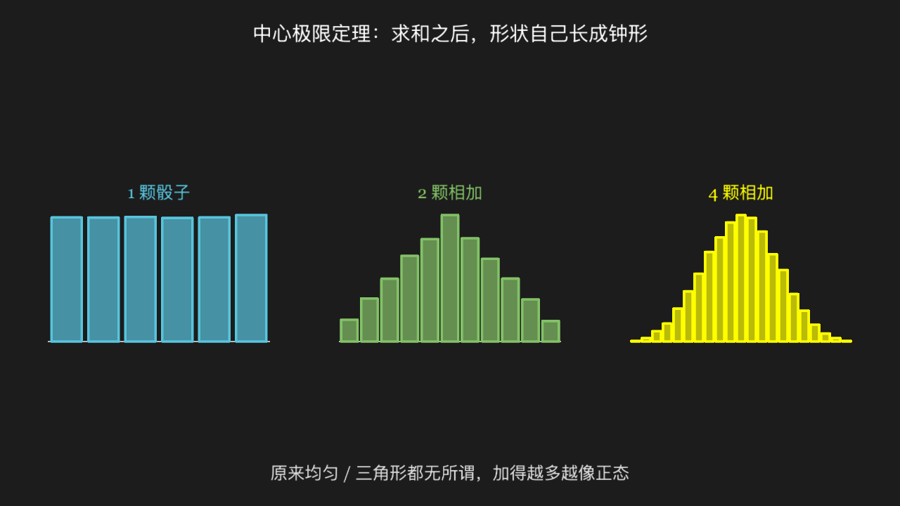
"""中心极限定理:独立同分布求和,分布形状必然向正态靠拢

@expect 三个并排直方图,从左到右分别是一颗骰子(平的)、两颗之和(三角形)、四颗之和(明显钟形);右侧两张的柱子朝中间堆、两端塌下去,且被归一化成同高以便比较形状。
@note 讲解要点:单颗骰子是完全均匀的,一点都不「正态」;但只要把若干独立同分布的变量加起来,中心就会长出钟形——不管原来是什么分布。这是正态分布无处不在的根源。
"""

from manim import *
import numpy as np


class CentralLimitScene(Scene):
    def construct(self):
        rng = np.random.default_rng(2026)
        samples = 20000

        def heights_for(k):
            rolls = rng.integers(1, 7, size=(samples, k)).sum(axis=1).tolist()
            counts = [0] * (6 * k - k + 1)
            for value in rolls:
                counts[value - k] += 1
            peak = max(counts)
            return [c / peak for c in counts]

        def make_panel(k, center, color):
            hs = heights_for(k)
            span = 3.5
            slot = span / len(hs)
            bars = VGroup()
            for i, h in enumerate(hs):
                bar = Rectangle(width=slot * 0.82, height=float(h) * 2.0, color=color)
                bar.set_fill(color, opacity=0.7)
                bar.move_to([center - span / 2 + slot * (i + 0.5), -1.4 + float(h), 0])
                bars.add(bar)
            return bars

        panel_cfg = [(1, -4.6, BLUE, "1 颗骰子"), (2, 0.0, GREEN, "2 颗相加"), (4, 4.6, YELLOW, "4 颗相加")]
        bars_all = VGroup()
        titles = VGroup()
        for k, center, color, name in panel_cfg:
            bars_all.add(make_panel(k, center, color))
            titles.add(Text(name, font_size=26, color=color).move_to([center, 0.95, 0]))

        baseline = VGroup(
            *[Line([c - 1.75, -1.4, 0], [c + 1.75, -1.4, 0], color=GRAY_B, stroke_width=2) for _, c, _, _ in panel_cfg]
        )

        title = Text("中心极限定理:求和之后,形状自己长成钟形", font_size=30).to_edge(UP, buff=0.35)
        caption = Text(
            "原来均匀 / 三角形都无所谓,加得越多越像正态",
            font_size=26,
            color=GRAY_A,
        ).to_edge(DOWN, buff=0.35)

        self.play(Write(title), Create(baseline), run_time=0.8)
        self.play(LaggedStart(*[FadeIn(p) for p in bars_all], lag_ratio=0.25), run_time=2.0)
        self.play(Write(titles), run_time=0.8)
        self.play(Write(caption), run_time=0.7)
        self.wait(0.4)
泊松分布:稀有事件在时间轴上的到达
一条时间轴上不均匀地散落着若干次到达时刻(事件不能重叠),旁边画出计数 k 的分布柱:k=2、3 附近最高,两端迅速衰减。
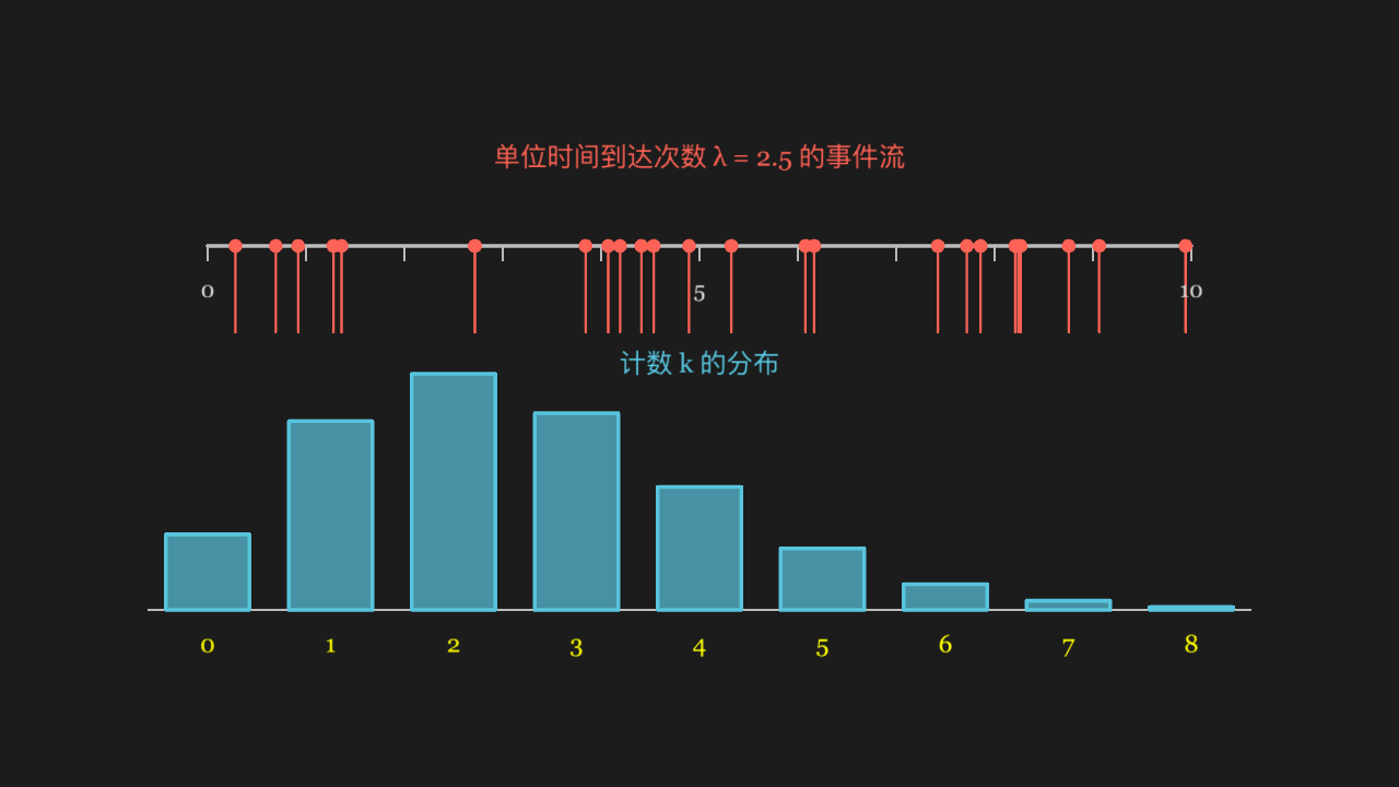
"""泊松分布:稀有事件在时间轴上的到达

@expect 一条时间轴上不均匀地散落着若干次到达时刻(事件不能重叠),旁边画出计数 k 的分布柱:k=2、3 附近最高,两端迅速衰减。
@note 讲解要点:泊松过程描述「单位时间内随机到达的稀有事件」——到达是独立的、速率恒定,于是计数服从泊松分布,它的期望和方差都等于 λ。
"""

from manim import *
import math
import numpy as np


class PoissonArrivalsScene(Scene):
    def construct(self):
        lam = 2.5
        length = 10.0
        rng = np.random.default_rng(7)

        gaps = rng.exponential(1.0 / lam, size=60)
        arrivals = np.cumsum(gaps)
        # 时间窗 [0, length] 线性映到数轴 [-5, 5]
        arrivals = arrivals[arrivals < length] - 5.0

        timeline = Line([-5.0, 1.5, 0], [5.0, 1.5, 0], color=GRAY_B, stroke_width=4)
        tick_labels = VGroup()
        for i in range(11):
            x = -5.0 + i
            tick_labels.add(Line([x, 1.5, 0], [x, 1.35, 0], color=GRAY_B, stroke_width=2))
            if i % 5 == 0:
                tick_labels.add(Text(str(i), font_size=22, color=GRAY_A).move_to([x, 1.05, 0]))

        drops = VGroup(
            *[
                Line([float(t), 1.5, 0], [float(t), 0.62, 0], color=RED, stroke_width=2.5) for t in arrivals
            ]
        )
        heads = VGroup(*[Dot([float(t), 1.5, 0], radius=0.07, color=RED) for t in arrivals])

        timeline_label = Text(f"单位时间到达次数 λ = {lam} 的事件流", font_size=26, color=RED)
        timeline_label.move_to([0, 2.4, 0])

        ks = list(range(0, 9))
        pmf = [float(np.exp(-lam) * lam ** k / math.factorial(k)) for k in ks]
        peak = max(pmf)
        bars = VGroup()
        labels_k = VGroup()
        for k, p in zip(ks, pmf):
            x = -5.0 + k * 1.25
            bar = Rectangle(width=0.85, height=p / peak * 2.4, color=BLUE)
            bar.set_fill(BLUE, opacity=0.7)
            bar.move_to([x, -2.2 + p / peak * 2.4 / 2, 0])
            bars.add(bar)
            labels_k.add(Text(str(k), font_size=24, color=YELLOW).move_to([x, -2.55, 0]))

        bar_axis = Line([-5.6, -2.2, 0], [5.6, -2.2, 0], color=GRAY_B, stroke_width=2)
        bar_label = Text("计数 k 的分布", font_size=26, color=BLUE).move_to([0, 0.3, 0])

        self.play(Write(timeline_label), Create(timeline), Create(tick_labels), run_time=0.9)
        self.play(LaggedStart(*[Create(d) for d in drops], lag_ratio=0.08), run_time=1.6)
        self.play(FadeIn(heads), run_time=0.5)
        self.play(Create(bar_axis), Write(bar_label), run_time=0.7)
        self.play(LaggedStart(*[FadeIn(b) for b in bars], lag_ratio=0.1), run_time=1.4)
        self.play(Write(labels_k), run_time=0.7)
        self.wait(0.4)
正态分布的 3σ 法则:钟形曲线下的面积怎么分
钟形曲线下方用虚线切出 ±1σ、±2σ、±3σ 三道关口,右侧列出各自覆盖的面积;下方 1000 次抽样的小点密密麻麻挤在中间,落在 ±2.5σ 之外的少数几个被染红。
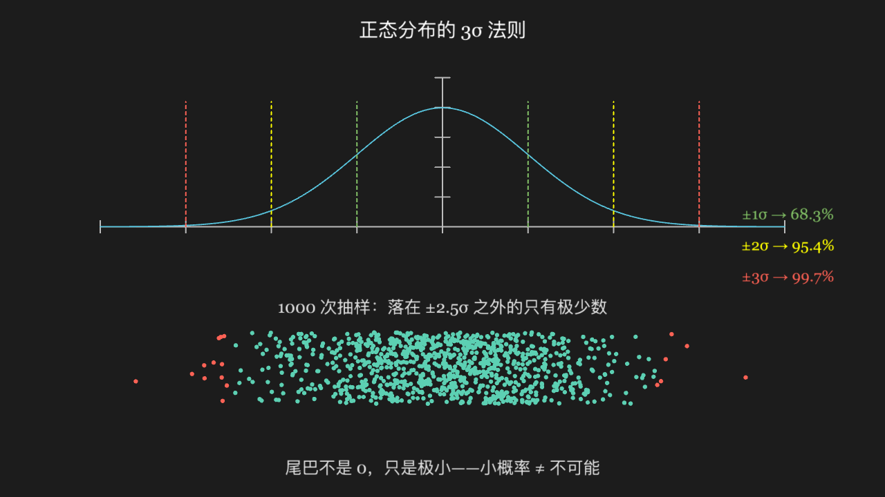
"""正态分布的 3σ 法则:钟形曲线下的面积怎么分

@expect 钟形曲线下方用虚线切出 ±1σ、±2σ、±3σ 三道关口,右侧列出各自覆盖的面积;下方 1000 次抽样的小点密密麻麻挤在中间,落在 ±2.5σ 之外的少数几个被染红。
@note 讲解要点:68.3% / 95.4% / 99.7% 说的是「概率集中在中心」,不是「值域到此为止」——尾巴永远存在,只是以小概率存在,所以 3σ 外的事件叫「小概率」而不叫「不可能」。
"""

from manim import *
import numpy as np


class NormalSigmaScene(Scene):
    def construct(self):
        rng = np.random.default_rng(31)
        pdf = lambda x: np.exp(-x * x / 2.0) / np.sqrt(2.0 * np.pi)

        ax = Axes(
            x_range=[-4, 4, 1],
            y_range=[0, 0.5, 0.1],
            x_length=11.0,
            y_length=2.4,
            tips=False,
            axis_config={"color": GRAY_B},
        )
        ax.shift(UP * 1.55)

        curve = ax.plot(lambda t: float(pdf(t)), x_range=[-4, 4], color=BLUE)

        gates = VGroup()
        for sigma, color in [(1.0, GREEN), (2.0, YELLOW), (3.0, RED)]:
            for sign in (-1, 1):
                gates.add(
                    DashedLine(
                        ax.c2p(sign * sigma, 0),
                        ax.c2p(sign * sigma, 0.42),
                        color=color,
                        stroke_width=2,
                    )
                )

        label_rows = VGroup(
            Text("±1σ → 68.3%", font_size=24, color=GREEN).move_to([5.55, 0.55, 0]),
            Text("±2σ → 95.4%", font_size=24, color=YELLOW).move_to([5.55, 0.05, 0]),
            Text("±3σ → 99.7%", font_size=24, color=RED).move_to([5.55, -0.45, 0]),
        )

        raw = rng.normal(0.0, 1.0, size=1000)
        ys = rng.uniform(-2.5, -1.35, size=1000)
        inside = VGroup()
        outside = VGroup()
        for value, y in zip(raw, ys):
            # 抽样点的 x 要过 c2p 换算,才和上方曲线同一个比例
            px = ax.c2p(float(value), 0)[0]
            if abs(value) > 2.5:
                outside.add(Dot([px, float(y), 0], radius=0.035, color=RED))
            else:
                inside.add(Dot([px, float(y), 0], radius=0.035, color=TEAL))

        sample_note = Text("1000 次抽样:落在 ±2.5σ 之外的只有极少数", font_size=26, color=GRAY_A)
        sample_note.move_to([0, -0.95, 0])

        title = Text("正态分布的 3σ 法则", font_size=30).to_edge(UP, buff=0.3)
        caption = Text("尾巴不是 0,只是极小——小概率 ≠ 不可能", font_size=26, color=GRAY_A)
        caption.to_edge(DOWN, buff=0.3)

        self.play(Write(title), Create(ax), run_time=0.8)
        self.play(Create(curve), run_time=1.2)
        self.play(Create(gates), Write(label_rows), run_time=1.0)
        self.play(LaggedStart(*[FadeIn(d) for d in inside], lag_ratio=0.002), run_time=1.6)
        self.play(FadeIn(outside), Write(sample_note), run_time=0.8)
        self.play(Write(caption), run_time=0.7)
        self.wait(0.4)
蒙特卡洛估算 π:往正方形里撒点,数落在四分之一圆内的比例
边长为 2 的正方形内含一个四分之一圆,蓝点在正方形里随机撒开:落在圆弧内的染黄、在外面的留蓝;右下角实时显示累计比例乘 4 逼近 3.14。
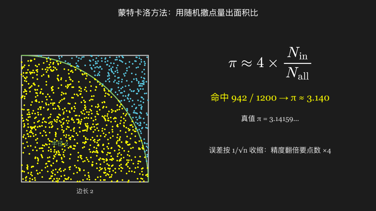
"""蒙特卡洛估算 π:往正方形里撒点,数落在四分之一圆内的比例

@expect 边长为 2 的正方形内含一个四分之一圆,蓝点在正方形里随机撒开:落在圆弧内的染黄、在外面的留蓝;右下角实时显示累计比例乘 4 逼近 3.14。
@note 讲解要点:P(落在圆内) = 圆面积/正方形面积 = π/4,所以 π ≈ 4 × 命中比例。随机模拟的误差按 1/√n 收缩,想把精度翻倍就得撒四倍的点。
"""

from manim import *
import numpy as np


class MonteCarloPiScene(Scene):
    def construct(self):
        rng = np.random.default_rng(1024)
        radius = 2.4
        # 圆心(四分之一圆的圆心在正方形左下角)
        cx, cy = -3.9, -0.5
        x0, y0 = cx + radius, cy + radius

        square = Rectangle(width=2 * radius, height=2 * radius, color=GRAY_B)
        square.move_to([cx, cy, 0])
        # 四分之一圆的半径 = 正方形边长(圆心在左下角,弧端点落在另外两个角上)。
        # Arc 以圆心为原点生成,shift 直接把圆心放到左下角——不能用 move_to(那挪的是外接框中心)
        arc = Arc(radius=2 * radius, start_angle=0, angle=PI / 2, color=GREEN, stroke_width=4)
        arc.shift([cx - radius, cy - radius, 0])

        side_label = Text("边长 2", font_size=22, color=GRAY_A).move_to([cx, cy - radius - 0.35, 0])
        # 标签沿弧的 45° 方向放在弧内,别压在点堆里
        arc_label = Text("半径 2", font_size=22, color=GREEN).move_to(
            [cx - radius + 1.45, cy - radius + 1.45, 0]
        )

        pts = rng.random((1200, 2))
        hits = VGroup()
        misses = VGroup()
        for u, v in pts:
            x = cx - radius + float(u) * 2 * radius
            y = cy - radius + float(v) * 2 * radius
            if u * u + v * v <= 1.0:
                hits.add(Dot([x, y, 0], radius=0.03, color=YELLOW))
            else:
                misses.add(Dot([x, y, 0], radius=0.03, color=BLUE))

        ratio = len(hits) / len(pts)
        estimate = 4.0 * ratio

        formula = MathTex(
            r"\pi \approx 4 \times \frac{N_{\text{in}}}{N_{\text{all}}}",
            font_size=54,
        ).move_to([3.1, 1.6, 0])

        result = Text(f"命中 {len(hits)} / {len(pts)} → π ≈ {estimate:.3f}", font_size=34, color=YELLOW)
        result.move_to([3.1, 0.3, 0])
        truth = Text("真值 π = 3.14159...", font_size=26, color=GRAY_A).move_to([3.1, -0.5, 0])

        error_note = Text("误差按 1/√n 收缩:精度翻倍要点数 ×4", font_size=26, color=GRAY_A)
        error_note.move_to([3.1, -1.7, 0])

        title = Text("蒙特卡洛方法:用随机撒点量出面积比", font_size=30).to_edge(UP, buff=0.3)

        self.play(Write(title), run_time=0.7)
        self.play(Create(square), Create(arc), Write(side_label), Write(arc_label), run_time=0.9)
        self.play(LaggedStart(*[FadeIn(d) for d in hits], lag_ratio=0.01), run_time=1.6)
        self.play(FadeIn(misses), run_time=0.8)
        self.play(Write(formula), run_time=0.8)
        self.play(Write(result), Write(truth), run_time=0.8)
        self.play(Write(error_note), run_time=0.7)
        self.wait(0.4)
随机游走:每一步无记忆,但整体呈现出 √n 的尺度
四条独立的一维随机游走轨迹同时从原点出发,各自上下乱走、互不同步;终点被标出,包围它们的横向包络宽度远小于步数——典型量级是 √n 而不是 n。
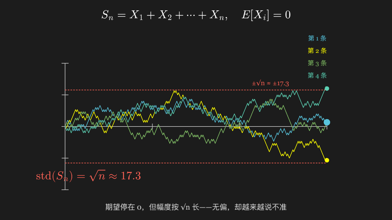
"""随机游走:每一步无记忆,但整体呈现出 √n 的尺度

@expect 四条独立的一维随机游走轨迹同时从原点出发,各自上下乱走、互不同步;终点被标出,包围它们的横向包络宽度远小于步数——典型量级是 √n 而不是 n。
@note 讲解要点:每一步的期望位移是 0,所以游走不会「漂」到某一边;但方差逐步累加,标准差按 √n 增长。这正是「无偏但不确定」的标准图像,也是扩散方程与布朗运动的离散原型。
"""

from manim import *
import numpy as np
import math


class RandomWalkScene(Scene):
    def construct(self):
        rng = np.random.default_rng(1234)
        steps = 300
        colors = [BLUE, YELLOW, GREEN, TEAL]

        ax = Axes(
            x_range=[0, 300, 100],
            y_range=[-30, 30, 15],
            x_length=9.5,
            y_length=4.6,
            tips=False,
            axis_config={"color": GRAY_B},
        )
        ax.shift(DOWN * 0.6)

        zero_line = DashedLine(ax.c2p(0, 0), ax.c2p(300, 0), color=GRAY_B, stroke_width=2)

        # ±√n 参考带:两端绝对坐标(c2p),直观对照「包络宽度 ~ √n 而非 n」
        sqrt_n = math.sqrt(300)
        band_top = DashedLine(ax.c2p(0, sqrt_n), ax.c2p(300, sqrt_n), color=RED, stroke_width=2)
        band_bottom = DashedLine(ax.c2p(0, -sqrt_n), ax.c2p(300, -sqrt_n), color=RED, stroke_width=2)
        band_label = Text("±√n ≈ ±17.3", font_size=24, color=RED).move_to([2.7, 0.98, 0])

        walks = VGroup()
        ends = VGroup()
        legend = VGroup()
        end_pts = []
        for idx, color in enumerate(colors):
            moves = rng.choice([-1.0, 1.0], size=steps)
            path_values = np.concatenate([[0.0], np.cumsum(moves)])
            pts = [ax.c2p(int(i), float(v)) for i, v in enumerate(path_values)]
            walks.add(
                VGroup(*[Line(pts[i], pts[i + 1], color=color, stroke_width=2) for i in range(len(pts) - 1)])
            )
            end_pts.append(pts[-1])
            ends.add(Dot(pts[-1], radius=0.08, color=color))
            legend.add(Text(f"第 {idx + 1} 条", font_size=22, color=color).move_to([4.4, 2.6 - idx * 0.45, 0]))
        # 蓝色终点单独补一颗稍大的点,避免与其他终点重叠后看不见
        blue_end_dot = Dot(end_pts[0], radius=0.11, color=BLUE, stroke_color=WHITE, stroke_width=1.5)

        sigma_note = MathTex(r"\text{std}(S_n) = \sqrt{n} \approx 17.3", font_size=40, color=RED)
        sigma_note.move_to([-3.9, -2.4, 0])
        formula = MathTex(r"S_n = X_1 + X_2 + \cdots + X_n,\quad E[X_i] = 0", font_size=40)
        formula.to_edge(UP, buff=0.35)
        caption = Text("期望停在 0,但幅度按 √n 长——无偏,却越来越说不准", font_size=26, color=GRAY_A)
        caption.to_edge(DOWN, buff=0.3)

        self.play(Write(formula), run_time=0.8)
        self.play(Create(ax), Create(zero_line), run_time=0.9)
        self.play(LaggedStart(*[Create(w) for w in walks], lag_ratio=0.3), run_time=3.0)
        self.play(FadeIn(ends), FadeIn(blue_end_dot), Write(legend), run_time=0.7)
        self.play(Create(band_top), Create(band_bottom), Write(band_label), run_time=0.8)
        self.play(Write(sigma_note), run_time=0.7)
        self.play(Write(caption), run_time=0.7)
        self.wait(0.4)
假设检验的两类错误:α 是弃真,β 是取伪
两条错开的钟形曲线分别代表原假设 H0 与备择假设 H1;H0 右尾被切出红线区(弃真 / 假阳性),H1 左尾被切出黄线区(取伪 / 假阴性),中间那道竖线就是拒绝域的门槛。
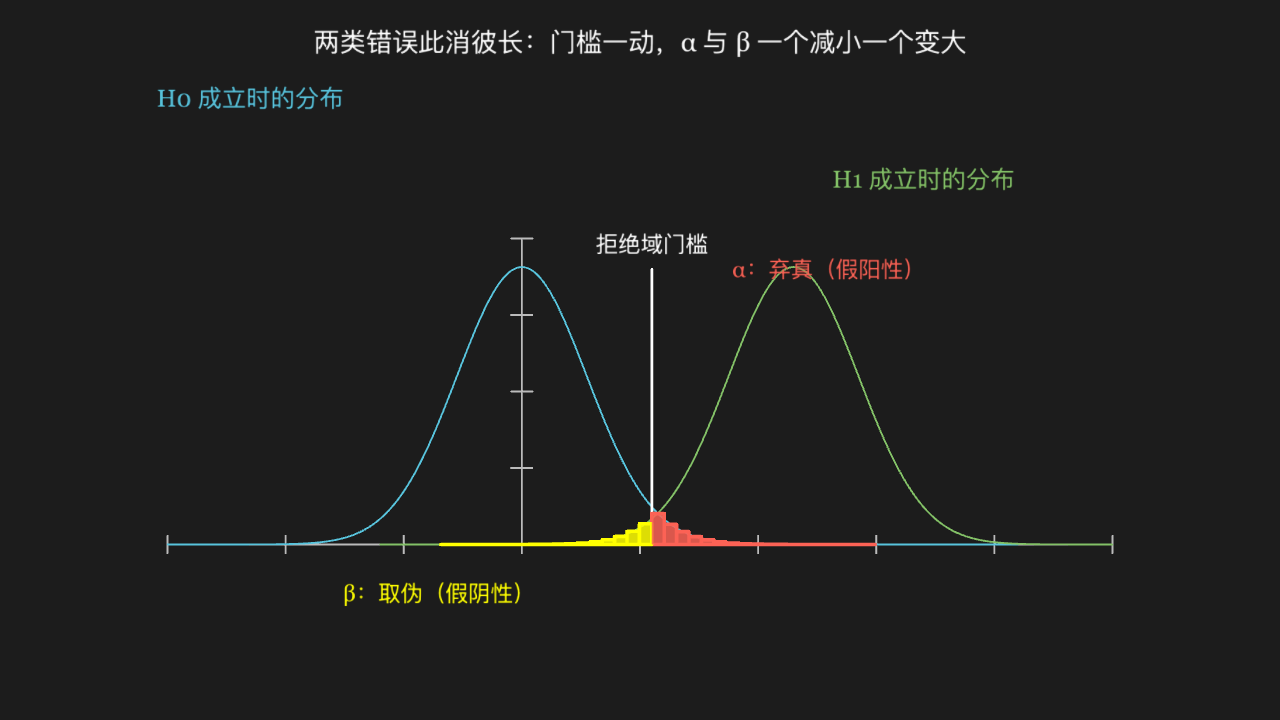
"""假设检验的两类错误:α 是弃真,β 是取伪

@expect 两条错开的钟形曲线分别代表原假设 H0 与备择假设 H1;H0 右尾被切出红线区(弃真 / 假阳性),H1 左尾被切出黄线区(取伪 / 假阴性),中间那道竖线就是拒绝域的门槛。
@note 讲解要点:门槛往右移,弃真概率 α 变小、但取伪概率 β 变大;两者此消彼长,不可能同时压到最低。只有加大样本量让两条曲线变瘦,才能同时把 α 和 β 都收小。
"""

from manim import *
import numpy as np


class HypothesisTestScene(Scene):
    def construct(self):
        pdf = lambda x, mu: np.exp(-(x - mu) ** 2 / (2 * 0.55 ** 2)) / (0.55 * np.sqrt(2 * np.pi))

        ax = Axes(
            x_range=[-3, 5, 1],
            y_range=[0, 0.8, 0.2],
            x_length=10.5,
            y_length=3.4,
            tips=False,
            axis_config={"color": GRAY_B},
        )
        ax.shift(DOWN * 0.35)

        critical = 1.1
        h0_mu = 0.0
        h1_mu = 2.3

        curve_h0 = ax.plot(lambda t: float(pdf(t, h0_mu)), x_range=[-3, 4.2], color=BLUE)
        curve_h1 = ax.plot(lambda t: float(pdf(t, h1_mu)), x_range=[-1.2, 5], color=GREEN)

        bar_span = (critical + 4.2) - critical
        bar_w = bar_span / 40.0
        alpha_bars = VGroup()
        for i in range(40):
            x = critical + bar_w * (i + 0.5)
            y_low = ax.c2p(0, 0)[1]
            y_high = ax.c2p(0, float(pdf(x, h0_mu)))[1]
            if abs(y_high - y_low) < 1e-6:
                continue
            bar = Rectangle(width=abs(ax.c2p(bar_w, 0)[0] - ax.c2p(0, 0)[0]), height=y_high - y_low, color=RED)
            bar.set_fill(RED, opacity=0.85)
            bar.move_to([ax.c2p(x, 0)[0], (y_low + y_high) / 2, 0])
            alpha_bars.add(bar)

        beta_bars = VGroup()
        for i in range(40):
            x = critical - bar_w * (i + 0.5)
            y_low = ax.c2p(0, 0)[1]
            y_high = ax.c2p(0, float(pdf(x, h1_mu)))[1]
            if abs(y_high - y_low) < 1e-6:
                continue
            bar = Rectangle(width=abs(ax.c2p(bar_w, 0)[0] - ax.c2p(0, 0)[0]), height=y_high - y_low, color=YELLOW)
            bar.set_fill(YELLOW, opacity=0.85)
            bar.move_to([ax.c2p(x, 0)[0], (y_low + y_high) / 2, 0])
            beta_bars.add(bar)

        gate = Line(ax.c2p(critical, 0), ax.c2p(critical, 0.72), color=WHITE, stroke_width=3)
        gate_label = Text("拒绝域门槛", font_size=24, color=WHITE).next_to(gate, UP, buff=0.12)

        labels = VGroup(
            Text("H0 成立时的分布", font_size=26, color=BLUE).move_to([ax.c2p(-2.3, 0)[0], 2.9, 0]),
            Text("H1 成立时的分布", font_size=26, color=GREEN).move_to([ax.c2p(3.4, 0)[0], 2.0, 0]),
            Text("α:弃真(假阳性)", font_size=24, color=RED).move_to([ax.c2p(2.6, 0)[0], 1.0, 0]),
            Text("β:取伪(假阴性)", font_size=24, color=YELLOW).move_to([ax.c2p(-0.7, 0)[0], -2.6, 0]),
        )

        title = Text("两类错误此消彼长:门槛一动,α 与 β 一个减小一个变大", font_size=28)
        title.to_edge(UP, buff=0.3)

        self.play(Write(title), Create(ax), run_time=0.8)
        self.play(Create(curve_h0), Create(curve_h1), run_time=1.4)
        self.play(Write(labels[0]), Write(labels[1]), run_time=0.7)
        self.play(Create(gate), Write(gate_label), run_time=0.6)
        self.play(FadeIn(alpha_bars), Write(labels[2]), run_time=0.9)
        self.play(FadeIn(beta_bars), Write(labels[3]), run_time=0.9)
        self.wait(0.4)