Calculus and analysis

Sequence limits, the squeeze theorem, Taylor expansion, the definition of e, the mean value theorem, upper and lower sums, accumulation functions, partial derivatives, gradient descent, double integrals, Fourier series and partial sums.

This page lists 12 examples. The code is imported from corpus/examples/math-calculus/; the screenshots are end states rendered on real machines.

Sequence limit: a_n = 1 + 1/n approaching 1

A row of points crowds denser as n grows and settles onto the dashed line y=1 without ever crossing it.

Rendered

Code

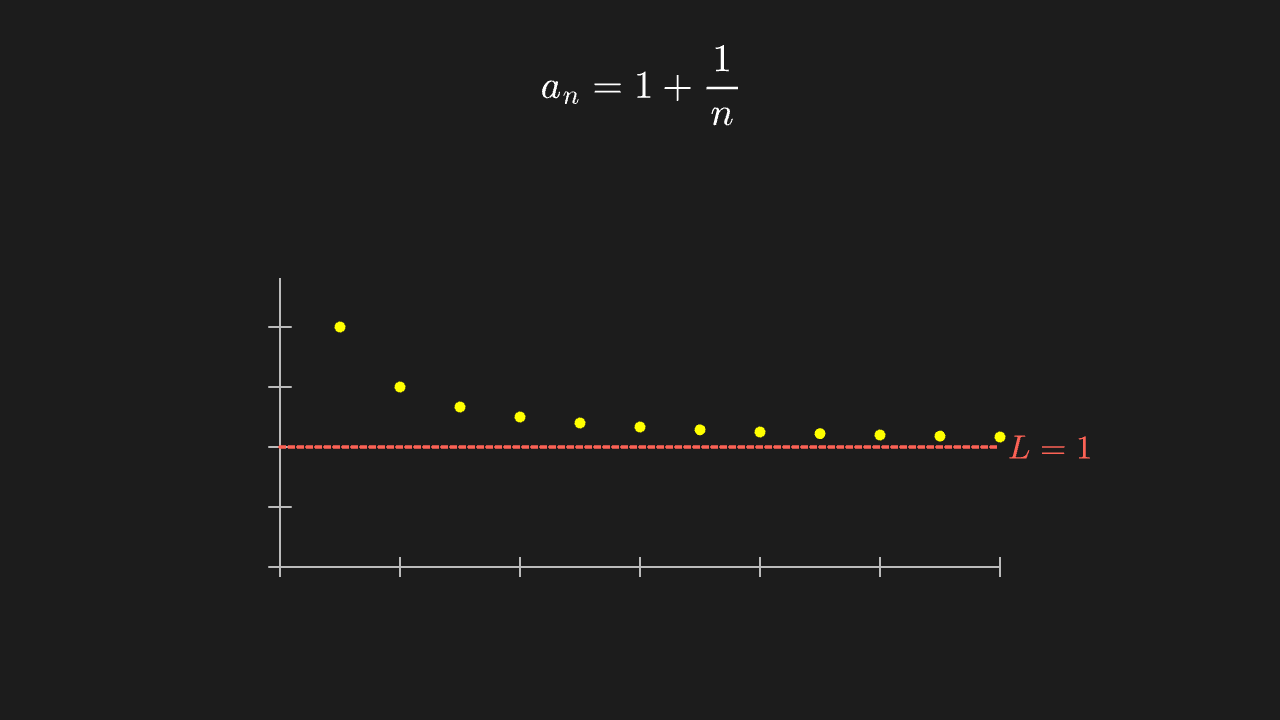
"""数列极限：a_n = 1 + 1/n 逼近 1

@expect 一排点随 n 增大越挤越密，逐渐贴上 y=1 那条虚线，但永远不与之相交。
@note 讲解要点：极限是「点在过程中趋近的那个值」，不是某一步取到的值——所以虚线画断的（取不到）。
"""

from manim import *


class SequenceLimitScene(Scene):
    def construct(self):
        ax = Axes(
            x_range=[0, 12, 2],
            y_range=[0, 2.4, 0.5],
            x_length=8.0,
            y_length=3.2,
            tips=False,
            axis_config={"color": GRAY_B},
        )
        ax.shift(DOWN * 0.7)

        limit_line = DashedLine(ax.c2p(0, 1), ax.c2p(12, 1), color=RED)
        limit_label = MathTex(r"L=1", color=RED, font_size=36).next_to(limit_line, RIGHT, buff=0.15)
        dots = VGroup(*[Dot(ax.c2p(n, 1 + 1 / n), radius=0.06, color=YELLOW) for n in range(1, 13)])
        formula = MathTex(r"a_n = 1 + \frac{1}{n}", font_size=42).to_edge(UP)

        self.play(Create(ax), Write(formula), run_time=1.0)
        self.play(Create(limit_line), Write(limit_label), run_time=0.6)
        self.play(LaggedStart(*[FadeIn(dot) for dot in dots], lag_ratio=0.12), run_time=2.0)
        self.play(Indicate(dots[11], color=RED), run_time=0.6)
        self.wait(0.4)

Squeeze theorem: x·sin(1/x) squeezed by ±x

The high-frequency oscillating curve in the middle stays between the two lines y=x and y=-x, and both ends collapse to the origin together.

Rendered

Code

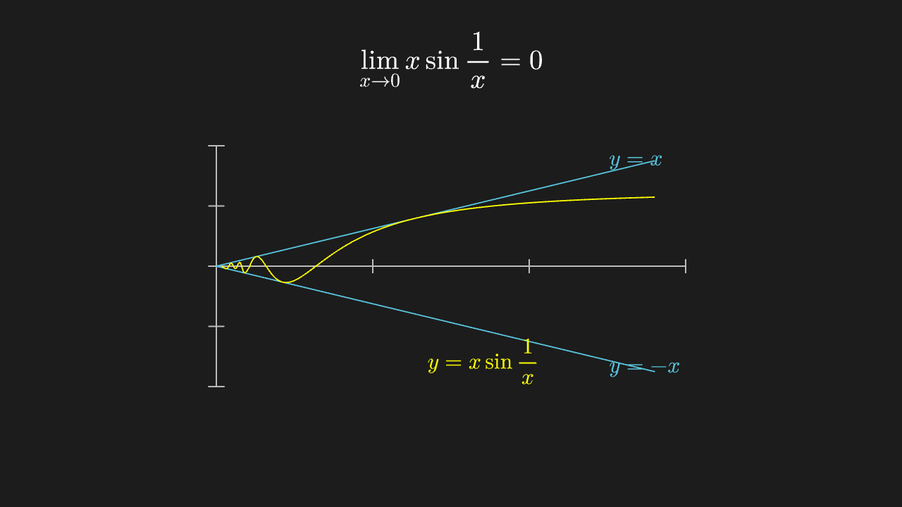
"""夹逼定理：x·sin(1/x) 被 ±x 夹住

@expect 中间那条高频抖动的曲线始终夹在两条直线（y=x 与 y=-x）之间，两端一起收到原点。
@note 讲解要点：抖得再厉害，只要被两条「同归于 0」的线夹住，极限就是 0——上下界比函数本身好算。
    从 0.02 起画：x→0 时 sin(1/x) 在有限采样下会漏峰，那是采样问题，不是曲线本身有界性变了。
"""

from manim import *
import numpy as np


class SqueezeTheoremScene(Scene):
    def construct(self):
        ax = Axes(
            x_range=[0, 1.5, 0.5],
            y_range=[-1.6, 1.6, 0.8],
            x_length=7.4,
            y_length=3.8,
            tips=False,
            axis_config={"color": GRAY_B},
        ).shift(DOWN * 0.2)

        upper = ax.plot(lambda x: x, x_range=[0, 1.4], color=BLUE)
        lower = ax.plot(lambda x: -x, x_range=[0, 1.4], color=BLUE)
        middle = ax.plot(lambda x: x * np.sin(1 / x), x_range=[0.02, 1.4], color=YELLOW)

        upper_label = MathTex(r"y=x", color=BLUE, font_size=34).next_to(ax.c2p(1.25, 1.25), UR, buff=0.05)
        lower_label = MathTex(r"y=-x", color=BLUE, font_size=34).next_to(ax.c2p(1.25, -1.25), DR, buff=0.05)
        middle_label = MathTex(r"y=x\sin\frac{1}{x}", color=YELLOW, font_size=34).next_to(ax.c2p(0.85, -0.75), DOWN, buff=0.25)
        title = MathTex(r"\lim_{x\to 0} x\sin\frac{1}{x} = 0", font_size=42).to_edge(UP)

        self.play(Create(ax), run_time=0.8)
        self.play(Create(upper), Create(lower), run_time=1.0)
        self.play(Write(upper_label), Write(lower_label), run_time=0.5)
        self.play(Create(middle), run_time=2.0)
        self.play(Write(middle_label), run_time=0.5)
        self.play(Write(title), run_time=0.8)
        self.play(Indicate(upper_label, color=WHITE), Indicate(lower_label, color=WHITE), run_time=0.7)
        self.wait(0.4)

Taylor expansion: polynomials approaching sin x order by order

The degree-1, 3, 5 and 7 polynomials each hug the sine curve more closely, matching first near the origin and diverging farther away; the formula on the right grows term by term into the full polynomial (degrees 1 through 7, no term missing) and finally takes the colour of the degree-7 curve.

Rendered

Code

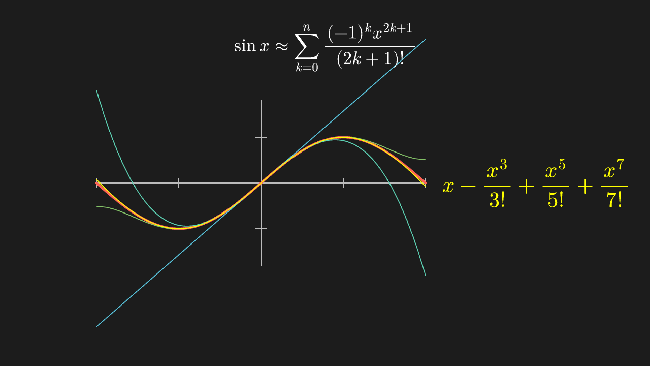
"""泰勒展开：多项式逐阶逼近 sin x

@expect 1 次、3 次、5 次、7 次多项式一条比一条贴近正弦曲线，在原点附近先贴合、越远越偏；
        右边那条公式逐阶补全为完整多项式（1 阶到 7 阶一项不缺），最终颜色与 7 阶曲线一致。
@note 讲解要点：阶数越高「贴合区间」越宽，但**每一阶都是往同一个点（原点）对齐**——远处永远靠不住。
    这是「局部逼近」最直观的画面：别指望用多项式在大范围上代替 sin。
"""

from manim import *
import math
import numpy as np


class TaylorSinScene(Scene):
    def construct(self):
        ax = Axes(
            x_range=[-PI, PI, PI / 2],
            y_range=[-1.8, 1.8, 1],
            x_length=7.2,
            y_length=3.6,
            tips=False,
            axis_config={"color": GRAY_B},
        ).shift(LEFT * 1.4)

        def taylor(terms):
            # sin x 的泰勒部分和：terms=1/2/3/4 分别是 1、3、5、7 阶
            def f(x):
                total = 0.0
                for k in range(terms):
                    total += (-1) ** k * x ** (2 * k + 1) / math.factorial(2 * k + 1)
                return total
            return f

        sine = ax.plot(lambda x: np.sin(x), x_range=[-PI, PI], color=RED, stroke_width=5)
        colors = [BLUE, TEAL, GREEN, YELLOW]
        # 每一阶新加的那一项；最终公式由这些项拼成完整的多项式
        parts = [r"x", r"-\frac{x^3}{3!}", r"+\frac{x^5}{5!}", r"+\frac{x^7}{7!}"]

        def make_formula(n_terms):
            tex = MathTex("".join(parts[:n_terms]), font_size=46)
            tex.set_color(colors[n_terms - 1])
            tex.move_to([4.6, 0, 0])
            return tex

        title = MathTex(r"\sin x \approx \sum_{k=0}^{n}\frac{(-1)^k x^{2k+1}}{(2k+1)!}", font_size=38).to_edge(UP)

        self.play(Create(ax), Write(title), run_time=1.0)
        self.play(Create(sine), run_time=1.0)
        formula = make_formula(1)
        first = ax.plot(taylor(1), x_range=[-PI, PI], color=colors[0])
        self.play(Create(first), Write(formula), run_time=0.9)
        for index in range(1, 4):
            curve = ax.plot(taylor(index + 1), x_range=[-PI, PI], color=colors[index])
            self.play(Create(curve), FadeOut(formula), run_time=0.7)
            formula = make_formula(index + 1)
            self.play(Write(formula), run_time=0.5)
        self.wait(0.4)

Definition of e: (1+1/n)^n increases monotonically towards e

The point sequence rises monotonically as n grows and always stays below the dashed line y=e.

Rendered

Code

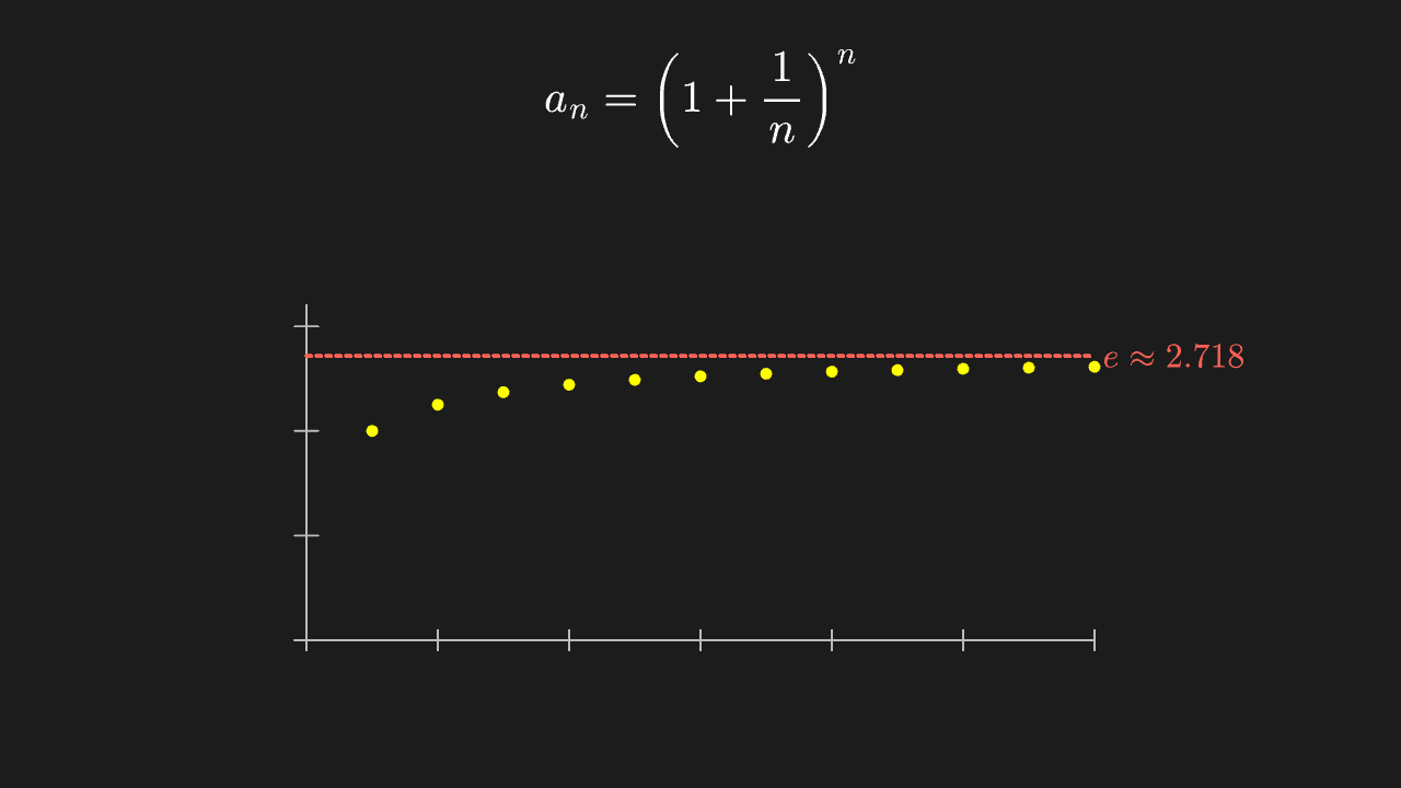
"""e 的定义：(1+1/n)^n 单调递增趋近 e

@expect 点列随 n 增大一路单调上升、并且始终待在那条 y=e 的虚线下面。
@note 讲解要点：与 1+1/n 那组对照着看——那组从上面压下来、这组从下面顶上去，两条都收敛，这就是 e。
    用 DecimalNumber 把 n 与当前值显示出来，比只看点更有说服力。
"""

from manim import *
import numpy as np


class EDefinitionScene(Scene):
    def construct(self):
        ax = Axes(
            x_range=[0, 12, 2],
            y_range=[0, 3.2, 1],
            x_length=8.0,
            y_length=3.4,
            tips=False,
            axis_config={"color": GRAY_B},
        )
        ax.shift(DOWN * 0.8)

        e_line = DashedLine(ax.c2p(0, np.e), ax.c2p(12, np.e), color=RED)
        e_label = MathTex(r"e \approx 2.718", color=RED, font_size=34).next_to(e_line, RIGHT, buff=0.15)
        dots = VGroup(*[Dot(ax.c2p(n, (1 + 1 / n) ** n), radius=0.06, color=YELLOW) for n in range(1, 13)])
        formula = MathTex(r"a_n = \left(1 + \frac{1}{n}\right)^n", font_size=44).to_edge(UP)

        self.play(Create(ax), Write(formula), run_time=1.0)
        self.play(Create(e_line), Write(e_label), run_time=0.6)
        self.play(LaggedStart(*[FadeIn(dot) for dot in dots], lag_ratio=0.12), run_time=2.0)
        self.play(Indicate(dots[11], color=RED), run_time=0.6)
        self.wait(0.4)

Lagrange mean value theorem: secant parallel to tangent

The chord through the endpoints (blue secant) is parallel to the tangent (yellow) at some interior point, and the tangency point lands exactly at the midpoint x=1.

Rendered

Code

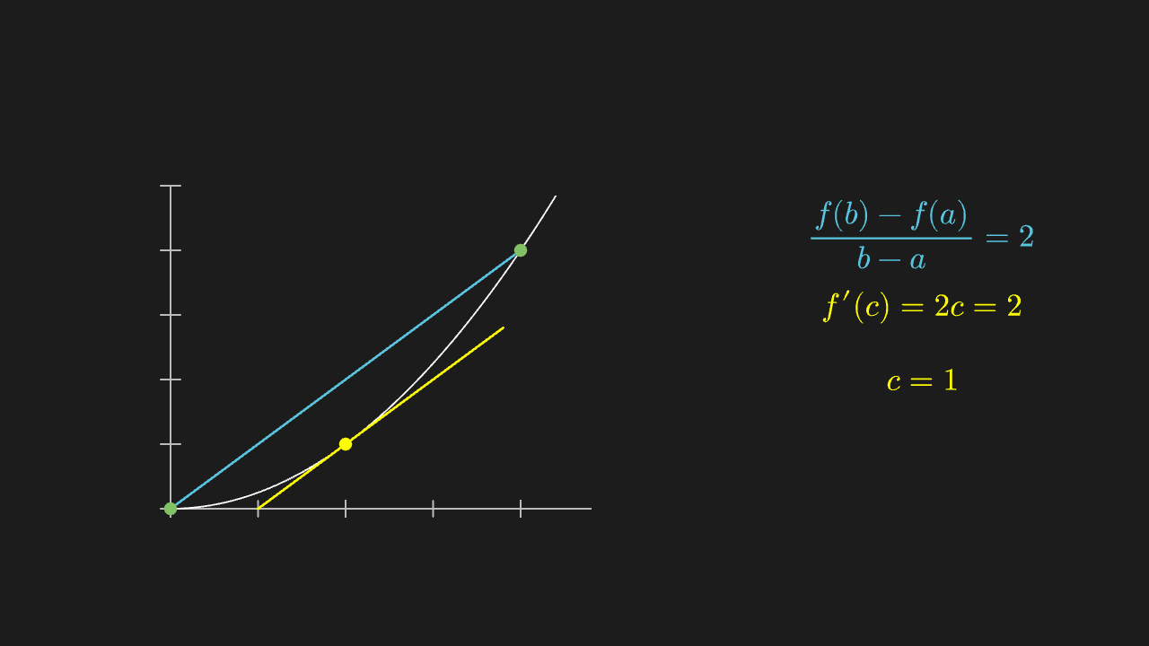
"""拉格朗日中值定理：割线与切线平行

@expect 两端连线（割线，蓝）与中间某点处的切线（黄）**平行**，切点恰好落在中点 x=1。
@note 讲解要点：平均变化率 = 某点瞬时变化率。对 f=x² 在 [0,2] 上，割线斜率 2 就是 x=1 处的导数——
    这就是「存在一点，其瞬时速度等于平均速度」的几何形状。
    两条公式各自 move_to 定位（不叠成 VGroup 再 arrange，见技能里那条「纯 MathTex 组别做几何查询」）。
"""

from manim import *


class MeanValueTheoremScene(Scene):
    def construct(self):
        ax = Axes(
            x_range=[0, 2.4, 0.5],
            y_range=[0, 5, 1],
            x_length=5.2,
            y_length=4.0,
            tips=False,
            axis_config={"color": GRAY_B},
        ).shift(LEFT * 2.4 + DOWN * 0.3)

        graph = ax.plot(lambda x: x ** 2, x_range=[0, 2.2], color=WHITE)
        point_a = Dot(ax.c2p(0, 0), color=GREEN)
        point_b = Dot(ax.c2p(2, 4), color=GREEN)
        chord = Line(ax.c2p(0, 0), ax.c2p(2, 4), color=BLUE)
        # 斜率 2 且过 (1,1) 的切线：y = 2x - 1，取 x∈[0.5, 1.9] 保证在框内
        tangent = Line(ax.c2p(0.5, 0), ax.c2p(1.9, 2.8), color=YELLOW)
        point_c = Dot(ax.c2p(1, 1), color=YELLOW)

        chord_slope = MathTex(r"\frac{f(b)-f(a)}{b-a} = 2", color=BLUE, font_size=38).move_to([4.3, 1.1, 0])
        derivative = MathTex(r"f'(c)=2c=2", color=YELLOW, font_size=38).move_to([4.3, 0.2, 0])
        answer = MathTex(r"c = 1", color=YELLOW, font_size=38).move_to([4.3, -0.7, 0])

        self.play(Create(ax), run_time=0.8)
        self.play(Create(graph), run_time=1.0)
        self.play(FadeIn(point_a), FadeIn(point_b), Create(chord), run_time=0.8)
        self.play(Write(chord_slope), run_time=0.6)
        self.play(Create(tangent), FadeIn(point_c), run_time=0.8)
        self.play(Write(derivative), run_time=0.5)
        self.play(Write(answer), run_time=0.5)
        self.play(Indicate(chord, color=BLUE), run_time=0.6)
        self.wait(0.4)

Upper and lower integrals: two sampling rules bracketing the true value

Left-endpoint (low) and right-endpoint (high) rectangle sets drawn on the same partition: the solid yellow blocks stay inside the curve while the top edges of the blue stroked frames stay above it; each set carries its label (upper sum / lower sum) so the comparison is immediate.

Rendered

Code

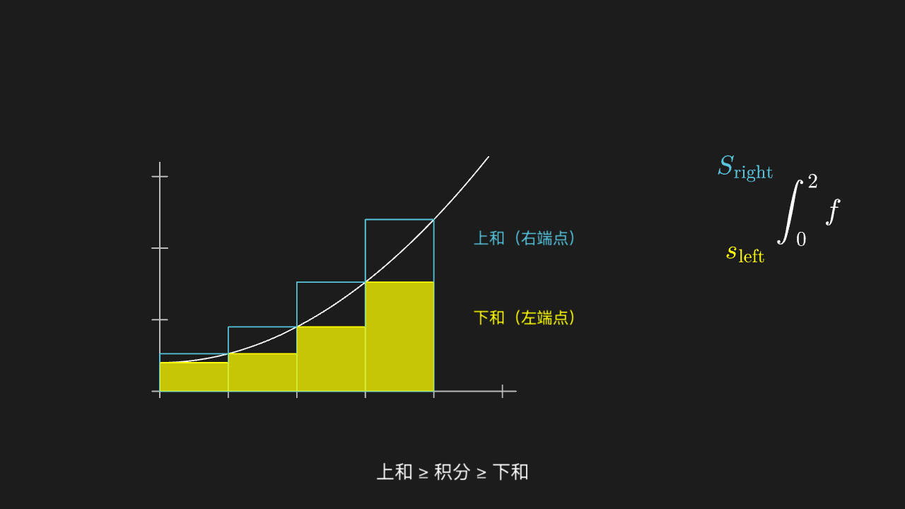
"""上积分与下积分：同一段区间两种取点法夹住真值

@expect 左端点（低）与右端点（高）两组矩形画在同一条分割上：黄色实心块始终在曲线内，蓝色描边框的顶边始终高出曲线；
        两组各带文字标注（上和 / 下和），对比一眼可见。
@note 讲解要点：两者都随 dx 变小而互相靠近，共同的极限就是定积分——「上和 ≥ 积分 ≥ 下和」。
    两条说明各自定位（纯 MathTex 组上做几何查询在我们没 KaTeX 的离线套件里会假报错）。
"""

from manim import *


class UpperLowerSumScene(Scene):
    def construct(self):
        ax = Axes(
            x_range=[0, 2.6, 0.5],
            y_range=[0, 3.2, 1],
            x_length=5.6,
            y_length=3.6,
            tips=False,
            axis_config={"color": GRAY_B},
        ).shift(LEFT * 1.8 + DOWN * 0.35)
        graph = ax.plot(lambda x: 0.5 * x * x + 0.4, x_range=[0, 2.4], color=WHITE)

        # 手工算坐标画矩形（与 Axes 的映射保持同一套常数），绕开几何查询
        # Axes 的 (0,0) 在其包围盒左下角：x 轴长 5.6、y 轴长 3.6，整体中心在 (-1.8, -0.35)
        x_unit = 5.6 / 2.6
        y_unit = 3.6 / 3.2
        origin = [-1.8 - x_unit * 1.3, -0.35 - y_unit * 1.6, 0]
        f = lambda x: 0.5 * x * x + 0.4

        def bar(x0, x1, h, color, fill_opacity):
            rect = Rectangle(width=(x1 - x0) * x_unit, height=h * y_unit, color=color, stroke_width=2)
            rect.set_fill(color, opacity=fill_opacity)
            rect.move_to([origin[0] + (x0 + x1) / 2 * x_unit, origin[1] + h * y_unit / 2, 0])
            return rect

        edges = [0.0, 0.5, 1.0, 1.5, 2.0]
        upper = VGroup(*[bar(edges[i], edges[i + 1], f(edges[i + 1]), BLUE, 0.0) for i in range(4)])
        lower = VGroup(*[bar(edges[i], edges[i + 1], f(edges[i]), YELLOW, 0.75) for i in range(4)])

        label_upper = Text("上和（右端点）", font_size=24, color=BLUE).move_to([1.2, 0.25, 0])
        label_lower = Text("下和（左端点）", font_size=24, color=YELLOW).move_to([1.2, -1.0, 0])
        high_label = MathTex(r"S_{\text{right}}", color=BLUE, font_size=40).move_to([4.6, 1.35, 0])
        low_label = MathTex(r"s_{\text{left}}", color=YELLOW, font_size=40).move_to([4.6, 0.0, 0])
        integral = MathTex(r"\int_0^2 f", font_size=44).move_to([5.6, 0.7, 0])
        caption = Text("上和 ≥ 积分 ≥ 下和", font_size=28).to_edge(DOWN, buff=0.4)

        self.play(Create(ax), Create(graph), run_time=1.0)
        self.play(FadeIn(lower), Write(label_lower), Write(low_label), run_time=0.8)
        self.play(Create(upper), Write(label_upper), Write(high_label), Write(integral), run_time=0.8)
        self.play(Write(caption), run_time=0.6)
        self.wait(0.4)

Accumulation function: the area function S(x) and its derivative

The area under the curve grows block by block to the right while the number S(x) on the right grows with it; at the end the page states S'(x)=f(x).

Rendered

Code

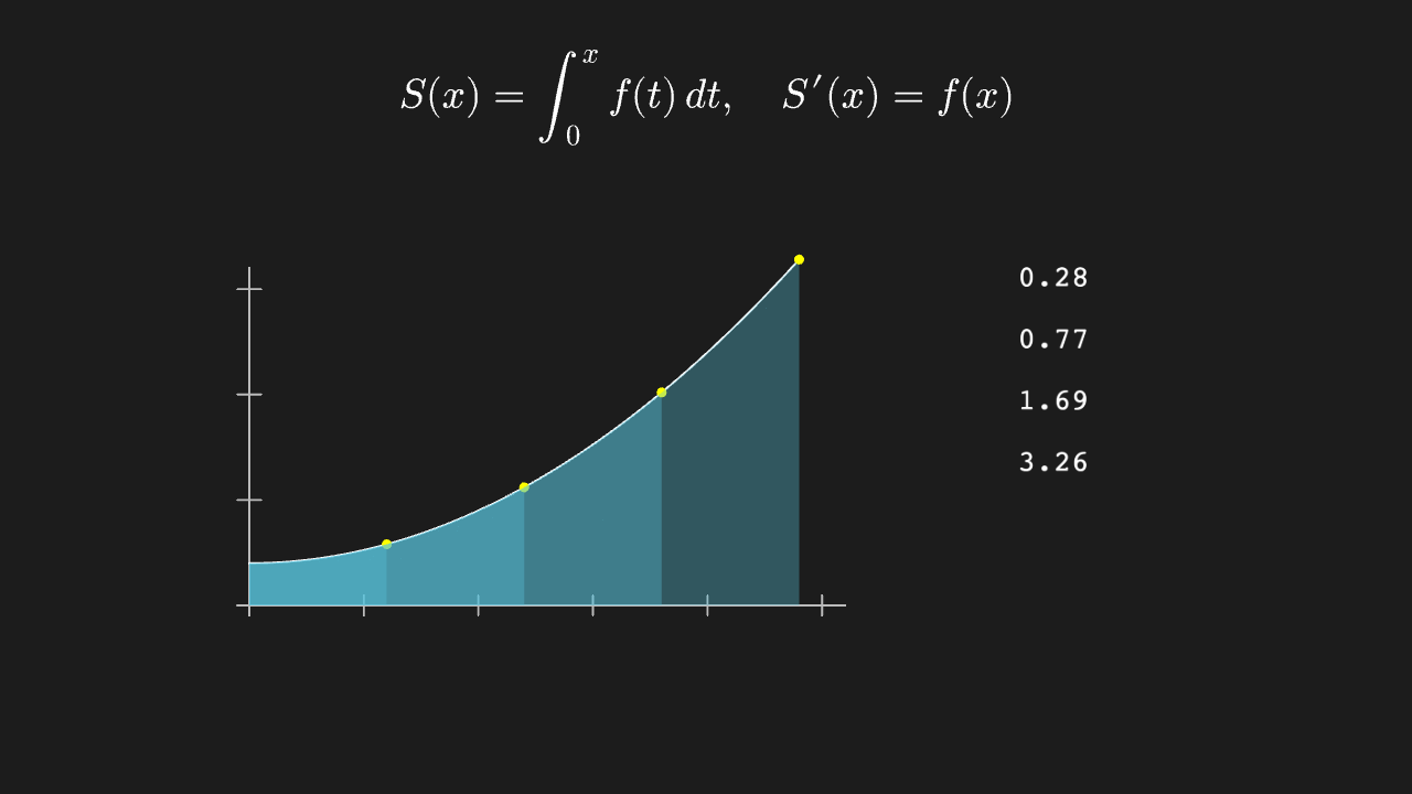
"""变上限积分：面积函数 S(x) 与它的导数

@expect 曲线下的面积一块块往右长出来，右侧数字 S(x) 同步变大；最后点明 S'(x)=f(x)。
@note 讲解要点：变上限积分是「一边走一边累加面积」，所以它的变化率就是被积函数本身——
    微积分基本定理的直观形状。这里用四个固定 x 逐块出现，不做连续滑动（画面上更容易看清每块的边界）。
"""

from manim import *


class AccumulationFunctionScene(Scene):
    def construct(self):
        ax = Axes(
            x_range=[0, 2.6, 0.5],
            y_range=[0, 3.2, 1],
            x_length=6.0,
            y_length=3.4,
            tips=False,
            axis_config={"color": GRAY_B},
        )
        ax.shift(LEFT * 1.6 + DOWN * 0.4)
        graph = ax.plot(lambda x: 0.5 * x * x + 0.4, x_range=[0, 2.4], color=WHITE)

        areas = VGroup(*[
            ax.get_area(graph, x_range=[0, x_stop], color=BLUE, opacity=0.35)
            for x_stop in [0.6, 1.2, 1.8, 2.4]
        ])
        markers = VGroup(*[
            Dot(ax.c2p(x_stop, 0.5 * x_stop ** 2 + 0.4), radius=0.05, color=YELLOW)
            for x_stop in [0.6, 1.2, 1.8, 2.4]
        ])
        values = VGroup(*[
            DecimalNumber(
                0.5 * x_stop ** 3 / 3 + 0.4 * x_stop, num_decimal_places=2, font_size=30,
            ).move_to([3.5, 1.2 - index * 0.62, 0])
            for index, x_stop in enumerate([0.6, 1.2, 1.8, 2.4])
        ])
        caption = MathTex(r"S(x)=\int_0^x f(t)\,dt,\quad S'(x)=f(x)", font_size=40).to_edge(UP)

        self.play(Create(ax), Create(graph), Write(caption), run_time=1.0)
        for index in range(4):
            self.play(FadeIn(areas[index]), FadeIn(markers[index]), FadeIn(values[index]), run_time=0.7)
        self.play(Indicate(caption, color=YELLOW), run_time=0.8)
        self.wait(0.4)

Partial derivatives: slopes seen with y fixed and with x fixed

The left panel draws how f changes with x at y=1 fixed, the right how f changes with y at x=1 fixed; each panel carries a yellow tangent through the point (1, 1.2), with slopes 0.8 and 1.6 — the right one visibly steeper.

Rendered

Code

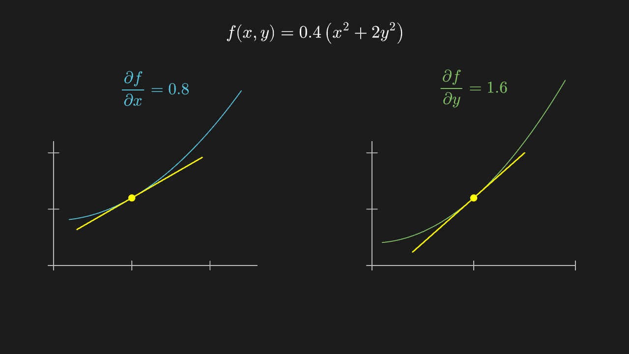
"""偏导数：分别固定 y 与固定 x 去看的斜率

@expect 左边那块画的是「固定 y=1 时 f 随 x 的变化」，右边是「固定 x=1 时 f 随 y 的变化」，
        两块各有一条过切点 (1, 1.2) 的黄色切线，斜率分别是 0.8 与 1.6，右边明显更陡。
@note 讲解要点：多元函数的「导数」得先说要沿哪个方向走——固定另一个变量，就退回一元情形。
    图上 f(x,y)=0.4(x²+2y²) 在点 (1,1)：f_x=0.8x=0.8、f_y=1.6y=1.6，所以右边明显更陡。
"""

from manim import *


class PartialDerivativeScene(Scene):
    def construct(self):
        left = Axes(x_range=[0, 2.6, 1], y_range=[0, 2.2, 1], x_length=4.6, y_length=2.8,
                    tips=False, axis_config={"color": GRAY_B}).shift(LEFT * 3.6 + DOWN * 0.6)
        right = Axes(x_range=[0, 2.0, 1], y_range=[0, 2.2, 1], x_length=4.6, y_length=2.8,
                     tips=False, axis_config={"color": GRAY_B}).shift(RIGHT * 3.6 + DOWN * 0.6)

        # 固定 y0=1：g(x) = 0.4*(x^2 + 2) → 在 x0=1 处切点 (1, 1.2)、斜率 f_x = 0.8*1 = 0.8
        # 切线 y = 1.2 + 0.8(x-1)：x=0.3 → 0.64，x=1.9 → 1.92
        cut_x = left.plot(lambda x: 0.4 * (x ** 2 + 2), x_range=[0.2, 2.4], color=BLUE)
        tan_x = Line(left.c2p(0.3, 0.64), left.c2p(1.9, 1.92), color=YELLOW)
        dot_x = Dot(left.c2p(1, 1.2), color=YELLOW)

        # 固定 x0=1：h(y) = 0.4*(1 + 2y^2) → 在 y0=1 处切点 (1, 1.2)、斜率 f_y = 1.6*1 = 1.6
        # 切线 y = 1.2 + 1.6(y-1)：y=0.4 → 0.24，y=1.5 → 2.0
        cut_y = right.plot(lambda y: 0.4 * (1 + 2 * y ** 2), x_range=[0.1, 1.9], color=GREEN)
        tan_y = Line(right.c2p(0.4, 0.24), right.c2p(1.5, 2.0), color=YELLOW)
        dot_y = Dot(right.c2p(1, 1.2), color=YELLOW)

        labels = VGroup(
            MathTex(r"\frac{\partial f}{\partial x} = 0.8", color=BLUE, font_size=36).move_to([-3.6, 2.0, 0]),
            MathTex(r"\frac{\partial f}{\partial y} = 1.6", color=GREEN, font_size=36).move_to([3.6, 2.0, 0]),
            MathTex(r"f(x,y)=0.4\left(x^2+2y^2\right)", font_size=38).to_edge(UP),
        )

        self.play(Write(labels[2]), run_time=0.8)
        self.play(Create(left), Create(cut_x), Write(labels[0]), run_time=1.0)
        self.play(Create(right), Create(cut_y), Write(labels[1]), run_time=1.0)
        self.play(Create(tan_x), FadeIn(dot_x), run_time=0.7)
        self.play(Create(tan_y), FadeIn(dot_y), run_time=0.7)
        self.wait(0.4)

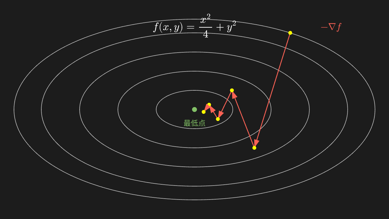
Gradient descent: stepping along the negative gradient towards the minimum

Five concentric ellipses are the contour lines (lower towards the centre); the polyline zigzags from the outer ring towards the centre — steps alternate on both sides of the valley along the negative gradient and shrink; arrows mark each step's direction.

Rendered

Code

"""梯度下降：沿负梯度方向一步步走向最小值

@expect 五条同心椭圆是等高线（越里越低），折线从外圈锯齿状折向中心——步子沿负梯度在谷的两侧交替弹跳、一步步收窄，箭头标出每一步的方向。
@note 讲解要点：等高线的法线方向就是梯度方向，所以「负梯度」总是垂直于当前等高线、指向更低的那一圈；
    步长 0.75 时 y 方向过冲（1-2·0.75<0），路径在谷两侧交替弹跳着收敛——「越到谷底走得越慢」的由来是梯度变小。
"""

from manim import *
import numpy as np


class GradientDescentScene(Scene):
    def construct(self):
        # f(x,y) = x^2/4 + y^2 的等高线：椭圆 x^2/4 + y^2 = r^2
        levels = VGroup(*[
            ParametricFunction(
                lambda t, r=r: [2 * r * np.cos(t), r * np.sin(t), 0],
                t_range=[0, TAU, 0.02],
                color=GRAY_B,
            )
            for r in [0.7, 1.4, 2.1, 2.8, 3.3]
        ])

        # 真实梯度下降：x ← x(1-α/2)、y ← y(1-2α)，α=0.75 时 y 过冲翻号，路径呈锯齿
        path_points = [
            [3.5, 2.8, 0],
            [3.5 * 0.625, 2.8 * -0.5, 0],
            [3.5 * 0.625**2, 2.8 * 0.25, 0],
            [3.5 * 0.625**3, 2.8 * -0.125, 0],
            [3.5 * 0.625**4, 2.8 * 0.0625, 0],
            [3.5 * 0.625**5, 2.8 * -0.03125, 0],
        ]
        dots = VGroup(*[Dot(point, radius=0.07, color=YELLOW) for point in path_points])
        arrows = VGroup(*[
            Arrow(path_points[index], path_points[index + 1], buff=0.12, color=RED, stroke_width=3)
            for index in range(len(path_points) - 1)
        ])
        center = Dot(ORIGIN, radius=0.09, color=GREEN)

        title = MathTex(r"f(x,y)=\frac{x^2}{4}+y^2", font_size=38).to_edge(UP)
        direction = MathTex(r"-\nabla f", color=RED, font_size=34).move_to([5.0, 3.0, 0])
        bottom_note = Text("最低点", font_size=26, color=GREEN).next_to(center, DOWN, buff=0.25)

        self.play(Create(levels), Write(title), run_time=1.0)
        self.play(FadeIn(center), Write(bottom_note), run_time=0.6)
        self.play(FadeIn(dots[0]), run_time=0.4)
        # dots[1:] 这种切片在适配层取不到子物体（下标才行），所以按下标走
        for index in range(len(arrows)):
            self.play(Create(arrows[index]), FadeIn(dots[index + 1]), run_time=0.6)
        self.play(Write(direction), run_time=0.5)
        self.wait(0.4)

Double integral: cutting the region into small squares

The rectangular region is tiled with small cells; cells inside the circle are highlighted and boundary cells count only partly.

Rendered

Code

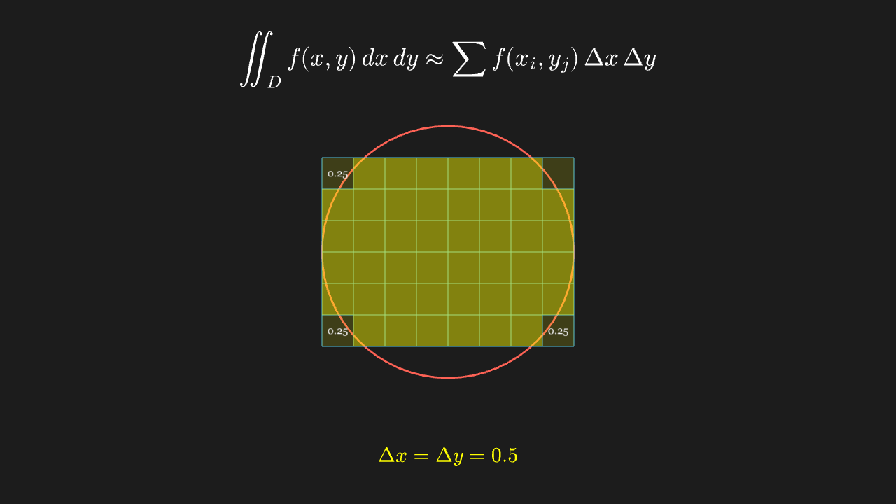
"""二重积分：把区域切成小方块

@expect 矩形区域内铺满小方格，落在圆内的格子被高亮，边上的格子只算一部分。
@note 讲解要点：二重积分就是「把区域切成很多小块、每块按 f 加权求和」的极限；格子越细越准。
    高亮用的是「格心在圆内」这一判据——这正是数值积分里最常用的采样方式。
"""

from manim import *
import numpy as np


class DoubleIntegralGridScene(Scene):
    def construct(self):
        dx, dy = 0.5, 0.5
        xs = np.arange(-2.0, 2.0, dx)
        ys = np.arange(-1.5, 1.5, dy)

        inside = VGroup()
        partial = VGroup()
        outside = VGroup()
        partial_cells = []
        for x0 in xs:
            for y0 in ys:
                cell = Rectangle(width=dx, height=dy, stroke_width=1)
                cell.move_to([float(x0) + dx / 2, float(y0) + dy / 2, 0])
                cx, cy = float(x0) + dx / 2, float(y0) + dy / 2
                r2 = cx ** 2 + cy ** 2
                if r2 <= 4.0:
                    cell.set_fill(YELLOW, 0.45)
                    inside.add(cell)
                else:
                    # 格心在外但方块与圆相交：四角至少一角落圆内，按角点比例估权重
                    corners = [(cx - dx / 2, cy - dy / 2), (cx + dx / 2, cy - dy / 2),
                               (cx - dx / 2, cy + dy / 2), (cx + dx / 2, cy + dy / 2)]
                    frac = sum(1.0 for ux, uy in corners if ux ** 2 + uy ** 2 <= 4.0) / 4.0
                    if frac > 0:
                        cell.set_fill(YELLOW, 0.15)
                        partial.add(cell)
                        partial_cells.append((cx, cy, frac))
                    else:
                        outside.add(cell)

        circle = Circle(radius=2.0, color=RED, stroke_width=3)
        weight_marks = VGroup()
        for cx, cy, frac in partial_cells[:3]:
            mark = Text(f"{frac:.2f}", font_size=16, color=WHITE)
            mark.move_to([cx, cy, 0])
            weight_marks.add(mark)
        labels = VGroup(
            MathTex(r"\iint_D f(x,y)\,dx\,dy \approx \sum f(x_i,y_j)\,\Delta x\,\Delta y", font_size=38).to_edge(UP),
            MathTex(r"\Delta x = \Delta y = 0.5", color=YELLOW, font_size=32).to_edge(DOWN, buff=0.6),
        )

        self.play(Write(labels[0]), run_time=0.8)
        self.play(Create(outside), Create(circle), run_time=1.0)
        self.play(LaggedStart(*[FadeIn(cell) for cell in inside], lag_ratio=0.02), run_time=1.6)
        self.play(FadeIn(partial), Write(weight_marks), run_time=0.8)
        self.play(Write(labels[1]), run_time=0.5)
        self.wait(0.4)

Fourier series approaching a square wave

A square wave (step-shaped) overlaid with four partial-sum curves: more terms make the flat parts flatter and the jumps steeper, yet a small overshoot always remains near each jump (the Gibbs phenomenon).

Rendered

Code

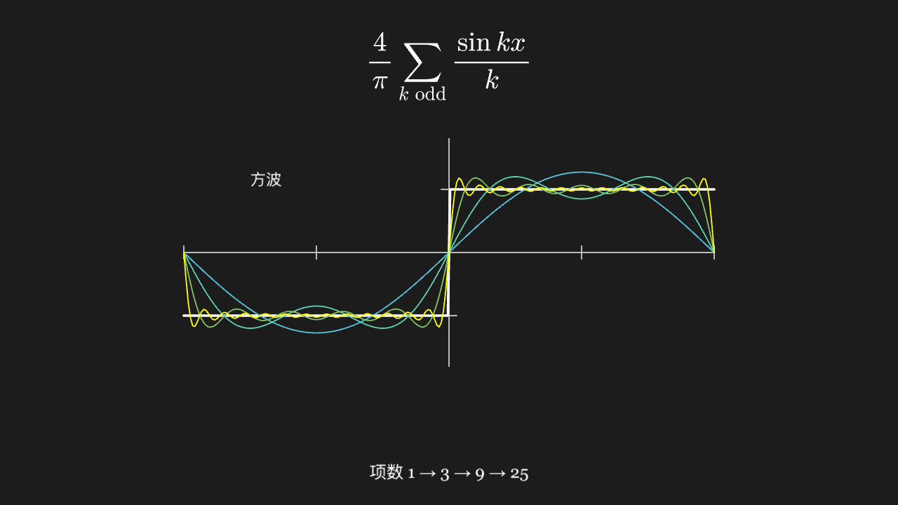
"""傅里叶级数逼近方波

@expect 一条方波（台阶状）与四条部分和曲线叠在一起：项数越多，平坦段越平、跳变处越陡，
        但跳变点附近始终有一个小过冲（吉布斯现象）。
@note 讲解要点：用正弦波叠出方波，需要无穷多项；有限项一定会「振铃」。
    部分和由 numpy 直接算好再交给 plot_line_graph——比在 lambda 里逐点求和快得多，也更稳。
"""

from manim import *
import numpy as np


class FourierSquareScene(Scene):
    def construct(self):
        ax = Axes(
            x_range=[-PI, PI, PI / 2],
            y_range=[-1.8, 1.8, 1],
            x_length=8.4,
            y_length=3.6,
            tips=False,
            axis_config={"color": GRAY_B},
        )
        xs = np.linspace(-np.pi, np.pi, 240)
        square = np.sign(np.sin(xs))
        square[square == 0] = 1.0

        square_graph = ax.plot_line_graph(xs, square, add_vertex_dots=False,
                                          line_color=WHITE, stroke_width=4)
        square_label = Text("方波", font_size=24, color=WHITE).move_to([-2.9, 1.15, 0])
        partials = VGroup()
        for terms, color in [(1, BLUE), (3, TEAL), (9, GREEN), (25, YELLOW)]:
            ys = np.zeros_like(xs)
            for k in range(1, terms + 1, 2):
                ys += (4 / np.pi) * np.sin(k * xs) / k
            partials.add(ax.plot_line_graph(xs, ys, add_vertex_dots=False, line_color=color))

        note = Text("项数 1 → 3 → 9 → 25", font_size=26, color=WHITE).to_edge(DOWN, buff=0.35)
        title = MathTex(r"\frac{4}{\pi}\sum_{k\ \text{odd}}\frac{\sin kx}{k}", font_size=42).to_edge(UP)

        self.play(Create(ax), Create(square_graph), Write(square_label), run_time=1.0)
        self.play(Write(title), run_time=0.8)
        for curve in partials:
            self.play(Create(curve), run_time=0.8)
        self.play(Write(note), run_time=0.5)
        self.wait(0.5)

Partial sums: harmonic series diverges vs Σ1/n² converges

The blue line (harmonic partial sums) climbs without levelling off; the yellow line (1/n² partial sums) flattens quickly and stops.

Rendered

Code

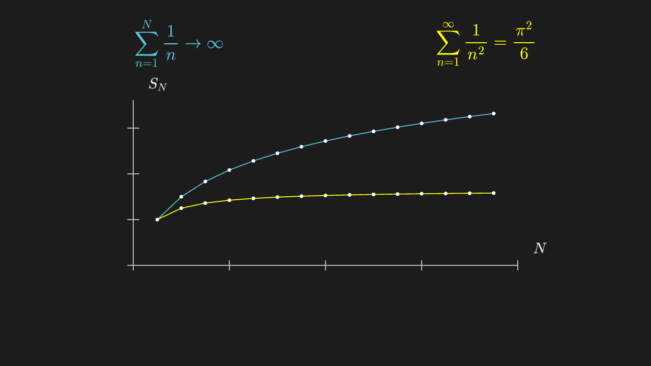
"""部分和：调和级数发散 vs Σ1/n² 收敛

@expect 蓝线（调和级数部分和）一路上爬、看不到头；黄线（1/n² 部分和）很快压平并停住。
@note 讲解要点：通项都趋于 0，但一个收敛一个发散——「通项趋于 0」只是必要条件。
    两条都用 plot_line_graph 画在 n 上，横轴就是项数。
"""

from manim import *
import numpy as np


class SeriesPartialSumScene(Scene):
    def construct(self):
        ax = Axes(
            x_range=[0, 16, 4],
            y_range=[0, 3.6, 1],
            x_length=8.4,
            y_length=3.6,
            tips=False,
            axis_config={"color": GRAY_B},
        )
        ns = np.arange(1, 16)
        harmonic = np.cumsum(1.0 / ns)
        quadratic = np.cumsum(1.0 / ns ** 2)

        harmonic_graph = ax.plot_line_graph(ns, harmonic, add_vertex_dots=True,
                                            line_color=BLUE, vertex_dot_radius=0.04)
        quadratic_graph = ax.plot_line_graph(ns, quadratic, add_vertex_dots=True,
                                            line_color=YELLOW, vertex_dot_radius=0.04)

        labels = VGroup(
            MathTex(r"\sum_{n=1}^{N}\frac{1}{n} \to \infty", color=BLUE, font_size=36).move_to([-3.2, 3.05, 0]),
            MathTex(r"\sum_{n=1}^{\infty}\frac{1}{n^2} = \frac{\pi^2}{6}", color=YELLOW, font_size=36).move_to([3.5, 3.05, 0]),
        )
        axis_labels = ax.get_axis_labels(x_label="N", y_label="S_N")

        self.play(Create(ax), Write(axis_labels), run_time=1.0)
        self.play(Write(labels[1]), Create(quadratic_graph), run_time=1.2)
        self.play(Write(labels[0]), Create(harmonic_graph), run_time=1.5)
        self.wait(0.4)