高等数学与数学分析

数列极限、夹逼、泰勒、e 的定义、中值定理、上下和、变上限积分、偏导、梯度下降、二重积分、傅里叶与级数。

本页 12 条示例。代码引自 corpus/examples/math-calculus/，截图为真机渲染的终态。

数列极限：a_n = 1 + 1/n 逼近 1

一排点随 n 增大越挤越密，逐渐贴上 y=1 那条虚线，但永远不与之相交。

画面

代码

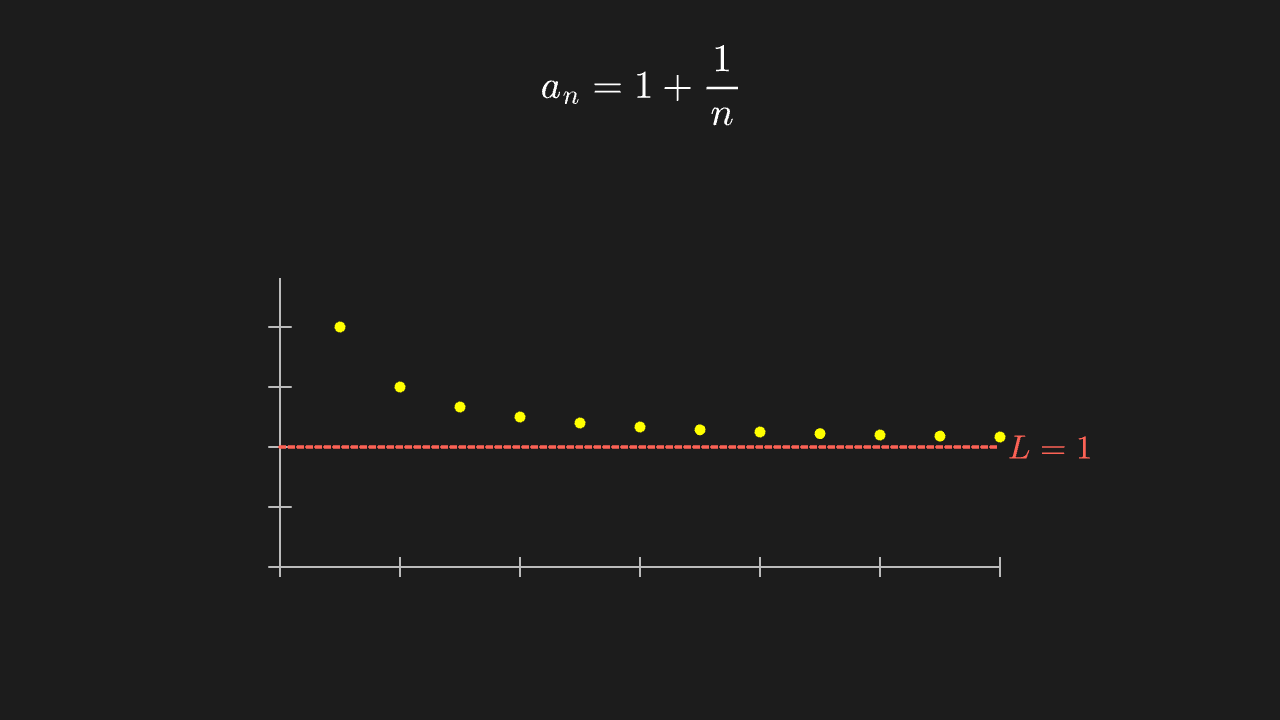
"""数列极限：a_n = 1 + 1/n 逼近 1

@expect 一排点随 n 增大越挤越密，逐渐贴上 y=1 那条虚线，但永远不与之相交。
@note 讲解要点：极限是「点在过程中趋近的那个值」，不是某一步取到的值——所以虚线画断的（取不到）。
"""

from manim import *


class SequenceLimitScene(Scene):
    def construct(self):
        ax = Axes(
            x_range=[0, 12, 2],
            y_range=[0, 2.4, 0.5],
            x_length=8.0,
            y_length=3.2,
            tips=False,
            axis_config={"color": GRAY_B},
        )
        ax.shift(DOWN * 0.7)

        limit_line = DashedLine(ax.c2p(0, 1), ax.c2p(12, 1), color=RED)
        limit_label = MathTex(r"L=1", color=RED, font_size=36).next_to(limit_line, RIGHT, buff=0.15)
        dots = VGroup(*[Dot(ax.c2p(n, 1 + 1 / n), radius=0.06, color=YELLOW) for n in range(1, 13)])
        formula = MathTex(r"a_n = 1 + \frac{1}{n}", font_size=42).to_edge(UP)

        self.play(Create(ax), Write(formula), run_time=1.0)
        self.play(Create(limit_line), Write(limit_label), run_time=0.6)
        self.play(LaggedStart(*[FadeIn(dot) for dot in dots], lag_ratio=0.12), run_time=2.0)
        self.play(Indicate(dots[11], color=RED), run_time=0.6)
        self.wait(0.4)

夹逼定理：x·sin(1/x) 被 ±x 夹住

中间那条高频抖动的曲线始终夹在两条直线（y=x 与 y=-x）之间，两端一起收到原点。

画面

代码

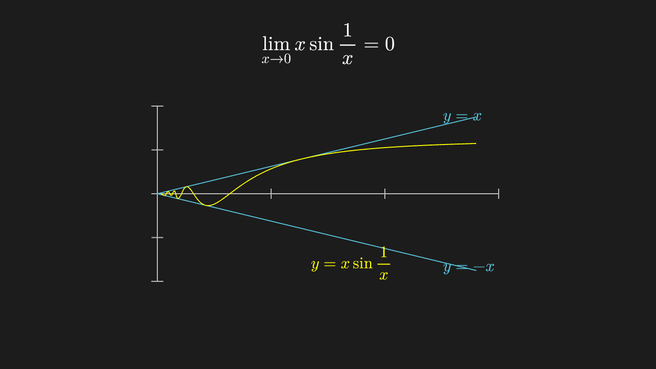
"""夹逼定理：x·sin(1/x) 被 ±x 夹住

@expect 中间那条高频抖动的曲线始终夹在两条直线（y=x 与 y=-x）之间，两端一起收到原点。
@note 讲解要点：抖得再厉害，只要被两条「同归于 0」的线夹住，极限就是 0——上下界比函数本身好算。
    从 0.02 起画：x→0 时 sin(1/x) 在有限采样下会漏峰，那是采样问题，不是曲线本身有界性变了。
"""

from manim import *
import numpy as np


class SqueezeTheoremScene(Scene):
    def construct(self):
        ax = Axes(
            x_range=[0, 1.5, 0.5],
            y_range=[-1.6, 1.6, 0.8],
            x_length=7.4,
            y_length=3.8,
            tips=False,
            axis_config={"color": GRAY_B},
        ).shift(DOWN * 0.2)

        upper = ax.plot(lambda x: x, x_range=[0, 1.4], color=BLUE)
        lower = ax.plot(lambda x: -x, x_range=[0, 1.4], color=BLUE)
        middle = ax.plot(lambda x: x * np.sin(1 / x), x_range=[0.02, 1.4], color=YELLOW)

        upper_label = MathTex(r"y=x", color=BLUE, font_size=34).next_to(ax.c2p(1.25, 1.25), UR, buff=0.05)
        lower_label = MathTex(r"y=-x", color=BLUE, font_size=34).next_to(ax.c2p(1.25, -1.25), DR, buff=0.05)
        middle_label = MathTex(r"y=x\sin\frac{1}{x}", color=YELLOW, font_size=34).next_to(ax.c2p(0.85, -0.75), DOWN, buff=0.25)
        title = MathTex(r"\lim_{x\to 0} x\sin\frac{1}{x} = 0", font_size=42).to_edge(UP)

        self.play(Create(ax), run_time=0.8)
        self.play(Create(upper), Create(lower), run_time=1.0)
        self.play(Write(upper_label), Write(lower_label), run_time=0.5)
        self.play(Create(middle), run_time=2.0)
        self.play(Write(middle_label), run_time=0.5)
        self.play(Write(title), run_time=0.8)
        self.play(Indicate(upper_label, color=WHITE), Indicate(lower_label, color=WHITE), run_time=0.7)
        self.wait(0.4)

泰勒展开：多项式逐阶逼近 sin x

1 次、3 次、5 次、7 次多项式一条比一条贴近正弦曲线，在原点附近先贴合、越远越偏；右边那条公式逐阶补全为完整多项式（1 阶到 7 阶一项不缺），最终颜色与 7 阶曲线一致。

画面

代码

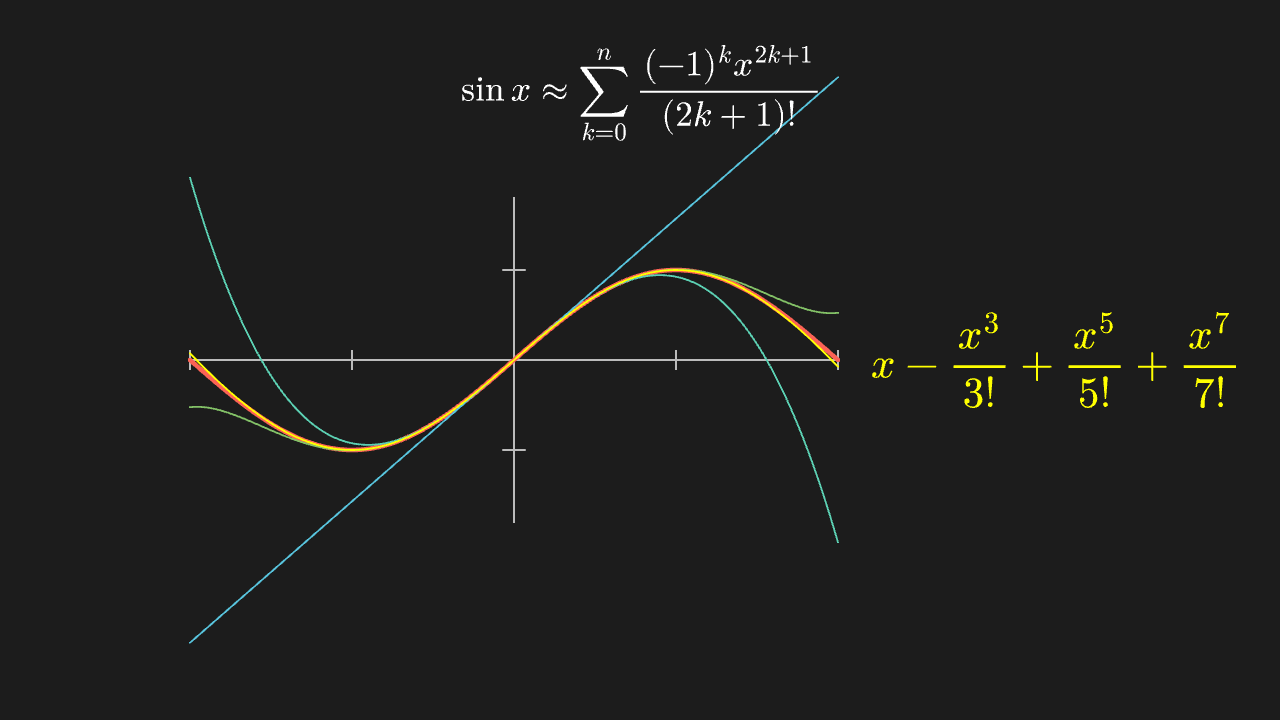
"""泰勒展开：多项式逐阶逼近 sin x

@expect 1 次、3 次、5 次、7 次多项式一条比一条贴近正弦曲线，在原点附近先贴合、越远越偏；
        右边那条公式逐阶补全为完整多项式（1 阶到 7 阶一项不缺），最终颜色与 7 阶曲线一致。
@note 讲解要点：阶数越高「贴合区间」越宽，但**每一阶都是往同一个点（原点）对齐**——远处永远靠不住。
    这是「局部逼近」最直观的画面：别指望用多项式在大范围上代替 sin。
"""

from manim import *
import math
import numpy as np


class TaylorSinScene(Scene):
    def construct(self):
        ax = Axes(
            x_range=[-PI, PI, PI / 2],
            y_range=[-1.8, 1.8, 1],
            x_length=7.2,
            y_length=3.6,
            tips=False,
            axis_config={"color": GRAY_B},
        ).shift(LEFT * 1.4)

        def taylor(terms):
            # sin x 的泰勒部分和：terms=1/2/3/4 分别是 1、3、5、7 阶
            def f(x):
                total = 0.0
                for k in range(terms):
                    total += (-1) ** k * x ** (2 * k + 1) / math.factorial(2 * k + 1)
                return total
            return f

        sine = ax.plot(lambda x: np.sin(x), x_range=[-PI, PI], color=RED, stroke_width=5)
        colors = [BLUE, TEAL, GREEN, YELLOW]
        # 每一阶新加的那一项；最终公式由这些项拼成完整的多项式
        parts = [r"x", r"-\frac{x^3}{3!}", r"+\frac{x^5}{5!}", r"+\frac{x^7}{7!}"]

        def make_formula(n_terms):
            tex = MathTex("".join(parts[:n_terms]), font_size=46)
            tex.set_color(colors[n_terms - 1])
            tex.move_to([4.6, 0, 0])
            return tex

        title = MathTex(r"\sin x \approx \sum_{k=0}^{n}\frac{(-1)^k x^{2k+1}}{(2k+1)!}", font_size=38).to_edge(UP)

        self.play(Create(ax), Write(title), run_time=1.0)
        self.play(Create(sine), run_time=1.0)
        formula = make_formula(1)
        first = ax.plot(taylor(1), x_range=[-PI, PI], color=colors[0])
        self.play(Create(first), Write(formula), run_time=0.9)
        for index in range(1, 4):
            curve = ax.plot(taylor(index + 1), x_range=[-PI, PI], color=colors[index])
            self.play(Create(curve), FadeOut(formula), run_time=0.7)
            formula = make_formula(index + 1)
            self.play(Write(formula), run_time=0.5)
        self.wait(0.4)

e 的定义：(1+1/n)^n 单调递增趋近 e

点列随 n 增大一路单调上升、并且始终待在那条 y=e 的虚线下面。

画面

代码

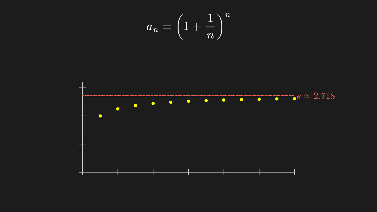
"""e 的定义：(1+1/n)^n 单调递增趋近 e

@expect 点列随 n 增大一路单调上升、并且始终待在那条 y=e 的虚线下面。
@note 讲解要点：与 1+1/n 那组对照着看——那组从上面压下来、这组从下面顶上去，两条都收敛，这就是 e。
    用 DecimalNumber 把 n 与当前值显示出来，比只看点更有说服力。
"""

from manim import *
import numpy as np


class EDefinitionScene(Scene):
    def construct(self):
        ax = Axes(
            x_range=[0, 12, 2],
            y_range=[0, 3.2, 1],
            x_length=8.0,
            y_length=3.4,
            tips=False,
            axis_config={"color": GRAY_B},
        )
        ax.shift(DOWN * 0.8)

        e_line = DashedLine(ax.c2p(0, np.e), ax.c2p(12, np.e), color=RED)
        e_label = MathTex(r"e \approx 2.718", color=RED, font_size=34).next_to(e_line, RIGHT, buff=0.15)
        dots = VGroup(*[Dot(ax.c2p(n, (1 + 1 / n) ** n), radius=0.06, color=YELLOW) for n in range(1, 13)])
        formula = MathTex(r"a_n = \left(1 + \frac{1}{n}\right)^n", font_size=44).to_edge(UP)

        self.play(Create(ax), Write(formula), run_time=1.0)
        self.play(Create(e_line), Write(e_label), run_time=0.6)
        self.play(LaggedStart(*[FadeIn(dot) for dot in dots], lag_ratio=0.12), run_time=2.0)
        self.play(Indicate(dots[11], color=RED), run_time=0.6)
        self.wait(0.4)

拉格朗日中值定理：割线与切线平行

两端连线（割线，蓝）与中间某点处的切线（黄）平行，切点恰好落在中点 x=1。

画面

代码

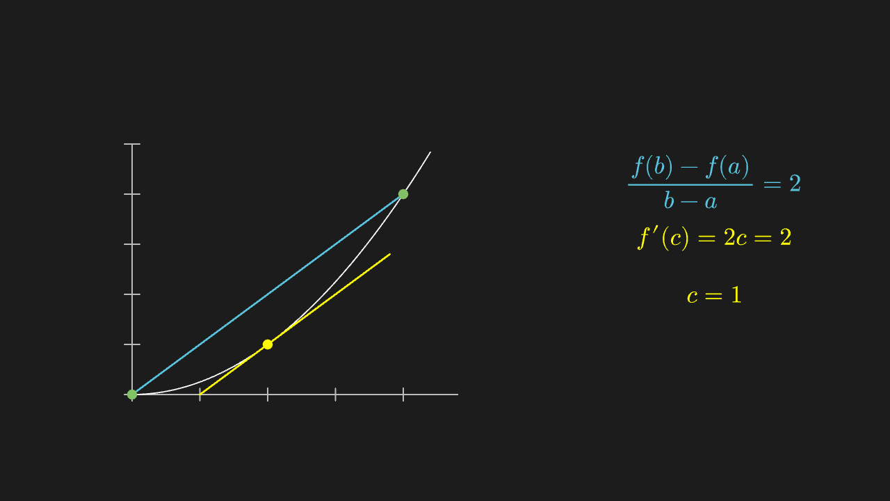
"""拉格朗日中值定理：割线与切线平行

@expect 两端连线（割线，蓝）与中间某点处的切线（黄）**平行**，切点恰好落在中点 x=1。
@note 讲解要点：平均变化率 = 某点瞬时变化率。对 f=x² 在 [0,2] 上，割线斜率 2 就是 x=1 处的导数——
    这就是「存在一点，其瞬时速度等于平均速度」的几何形状。
    两条公式各自 move_to 定位（不叠成 VGroup 再 arrange，见技能里那条「纯 MathTex 组别做几何查询」）。
"""

from manim import *


class MeanValueTheoremScene(Scene):
    def construct(self):
        ax = Axes(
            x_range=[0, 2.4, 0.5],
            y_range=[0, 5, 1],
            x_length=5.2,
            y_length=4.0,
            tips=False,
            axis_config={"color": GRAY_B},
        ).shift(LEFT * 2.4 + DOWN * 0.3)

        graph = ax.plot(lambda x: x ** 2, x_range=[0, 2.2], color=WHITE)
        point_a = Dot(ax.c2p(0, 0), color=GREEN)
        point_b = Dot(ax.c2p(2, 4), color=GREEN)
        chord = Line(ax.c2p(0, 0), ax.c2p(2, 4), color=BLUE)
        # 斜率 2 且过 (1,1) 的切线：y = 2x - 1，取 x∈[0.5, 1.9] 保证在框内
        tangent = Line(ax.c2p(0.5, 0), ax.c2p(1.9, 2.8), color=YELLOW)
        point_c = Dot(ax.c2p(1, 1), color=YELLOW)

        chord_slope = MathTex(r"\frac{f(b)-f(a)}{b-a} = 2", color=BLUE, font_size=38).move_to([4.3, 1.1, 0])
        derivative = MathTex(r"f'(c)=2c=2", color=YELLOW, font_size=38).move_to([4.3, 0.2, 0])
        answer = MathTex(r"c = 1", color=YELLOW, font_size=38).move_to([4.3, -0.7, 0])

        self.play(Create(ax), run_time=0.8)
        self.play(Create(graph), run_time=1.0)
        self.play(FadeIn(point_a), FadeIn(point_b), Create(chord), run_time=0.8)
        self.play(Write(chord_slope), run_time=0.6)
        self.play(Create(tangent), FadeIn(point_c), run_time=0.8)
        self.play(Write(derivative), run_time=0.5)
        self.play(Write(answer), run_time=0.5)
        self.play(Indicate(chord, color=BLUE), run_time=0.6)
        self.wait(0.4)

上积分与下积分：同一段区间两种取点法夹住真值

左端点（低）与右端点（高）两组矩形画在同一条分割上：黄色实心块始终在曲线内，蓝色描边框的顶边始终高出曲线；两组各带文字标注（上和 / 下和），对比一眼可见。

画面

代码

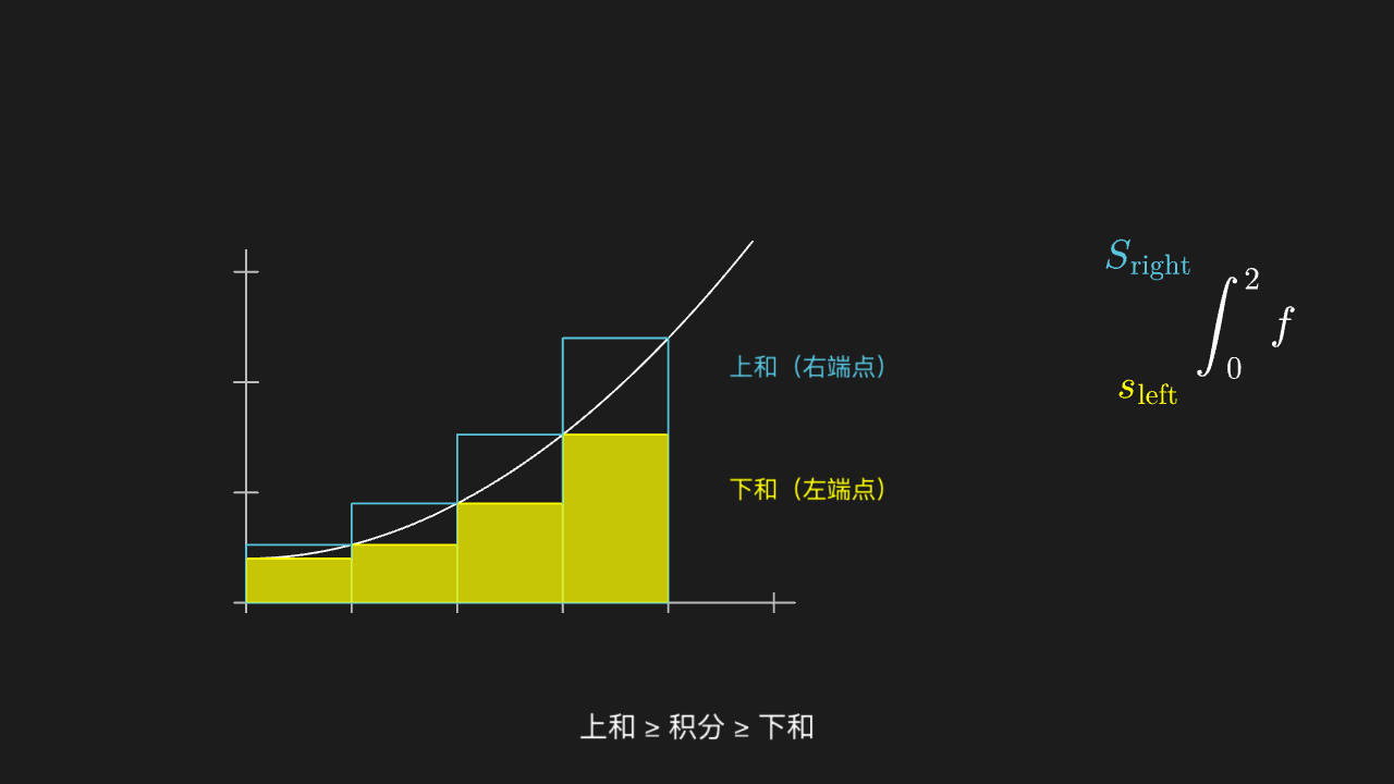
"""上积分与下积分：同一段区间两种取点法夹住真值

@expect 左端点（低）与右端点（高）两组矩形画在同一条分割上：黄色实心块始终在曲线内，蓝色描边框的顶边始终高出曲线；
        两组各带文字标注（上和 / 下和），对比一眼可见。
@note 讲解要点：两者都随 dx 变小而互相靠近，共同的极限就是定积分——「上和 ≥ 积分 ≥ 下和」。
    两条说明各自定位（纯 MathTex 组上做几何查询在我们没 KaTeX 的离线套件里会假报错）。
"""

from manim import *


class UpperLowerSumScene(Scene):
    def construct(self):
        ax = Axes(
            x_range=[0, 2.6, 0.5],
            y_range=[0, 3.2, 1],
            x_length=5.6,
            y_length=3.6,
            tips=False,
            axis_config={"color": GRAY_B},
        ).shift(LEFT * 1.8 + DOWN * 0.35)
        graph = ax.plot(lambda x: 0.5 * x * x + 0.4, x_range=[0, 2.4], color=WHITE)

        # 手工算坐标画矩形（与 Axes 的映射保持同一套常数），绕开几何查询
        # Axes 的 (0,0) 在其包围盒左下角：x 轴长 5.6、y 轴长 3.6，整体中心在 (-1.8, -0.35)
        x_unit = 5.6 / 2.6
        y_unit = 3.6 / 3.2
        origin = [-1.8 - x_unit * 1.3, -0.35 - y_unit * 1.6, 0]
        f = lambda x: 0.5 * x * x + 0.4

        def bar(x0, x1, h, color, fill_opacity):
            rect = Rectangle(width=(x1 - x0) * x_unit, height=h * y_unit, color=color, stroke_width=2)
            rect.set_fill(color, opacity=fill_opacity)
            rect.move_to([origin[0] + (x0 + x1) / 2 * x_unit, origin[1] + h * y_unit / 2, 0])
            return rect

        edges = [0.0, 0.5, 1.0, 1.5, 2.0]
        upper = VGroup(*[bar(edges[i], edges[i + 1], f(edges[i + 1]), BLUE, 0.0) for i in range(4)])
        lower = VGroup(*[bar(edges[i], edges[i + 1], f(edges[i]), YELLOW, 0.75) for i in range(4)])

        label_upper = Text("上和（右端点）", font_size=24, color=BLUE).move_to([1.2, 0.25, 0])
        label_lower = Text("下和（左端点）", font_size=24, color=YELLOW).move_to([1.2, -1.0, 0])
        high_label = MathTex(r"S_{\text{right}}", color=BLUE, font_size=40).move_to([4.6, 1.35, 0])
        low_label = MathTex(r"s_{\text{left}}", color=YELLOW, font_size=40).move_to([4.6, 0.0, 0])
        integral = MathTex(r"\int_0^2 f", font_size=44).move_to([5.6, 0.7, 0])
        caption = Text("上和 ≥ 积分 ≥ 下和", font_size=28).to_edge(DOWN, buff=0.4)

        self.play(Create(ax), Create(graph), run_time=1.0)
        self.play(FadeIn(lower), Write(label_lower), Write(low_label), run_time=0.8)
        self.play(Create(upper), Write(label_upper), Write(high_label), Write(integral), run_time=0.8)
        self.play(Write(caption), run_time=0.6)
        self.wait(0.4)

变上限积分：面积函数 S(x) 与它的导数

曲线下的面积一块块往右长出来，右侧数字 S(x) 同步变大；最后点明 S'(x)=f(x)。

画面

代码

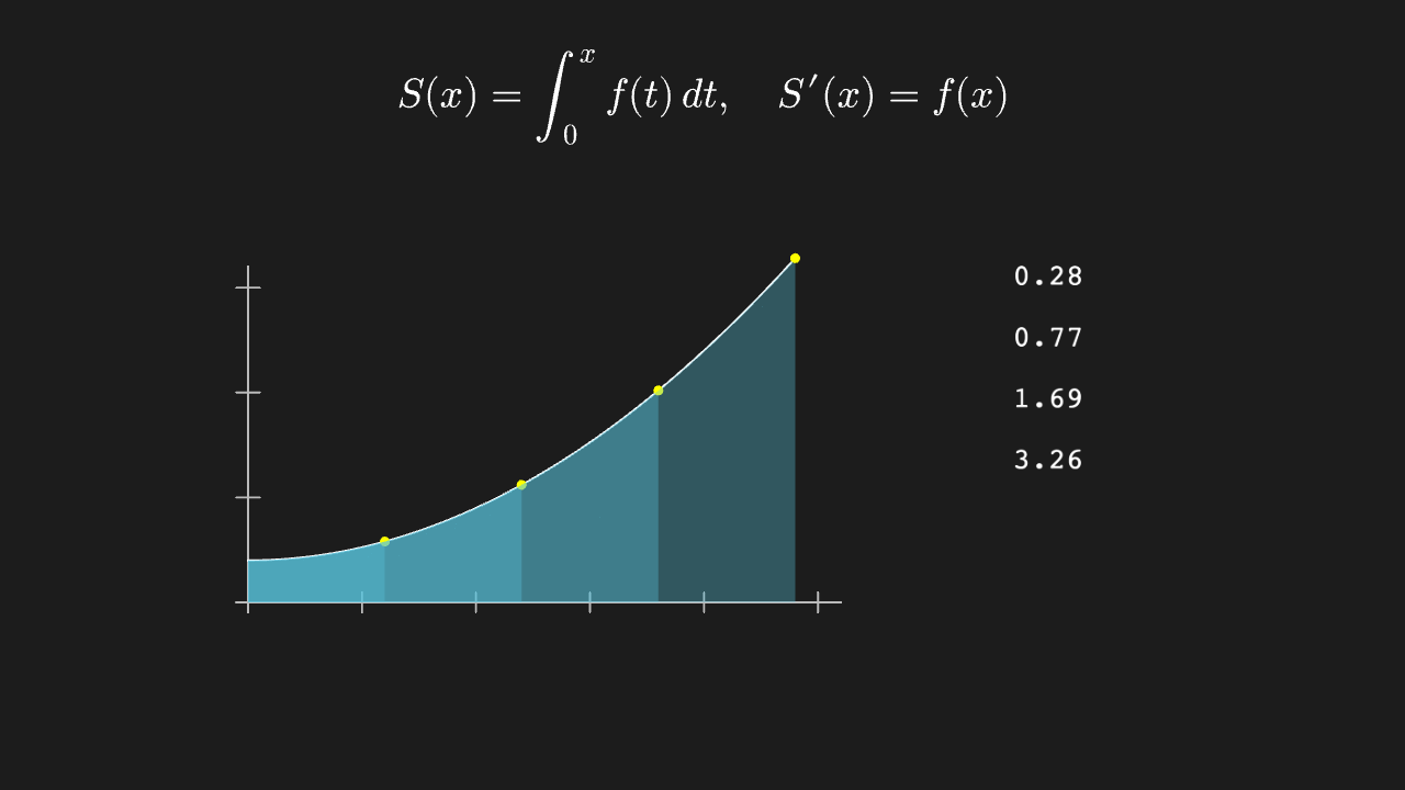
"""变上限积分：面积函数 S(x) 与它的导数

@expect 曲线下的面积一块块往右长出来，右侧数字 S(x) 同步变大；最后点明 S'(x)=f(x)。
@note 讲解要点：变上限积分是「一边走一边累加面积」，所以它的变化率就是被积函数本身——
    微积分基本定理的直观形状。这里用四个固定 x 逐块出现，不做连续滑动（画面上更容易看清每块的边界）。
"""

from manim import *


class AccumulationFunctionScene(Scene):
    def construct(self):
        ax = Axes(
            x_range=[0, 2.6, 0.5],
            y_range=[0, 3.2, 1],
            x_length=6.0,
            y_length=3.4,
            tips=False,
            axis_config={"color": GRAY_B},
        )
        ax.shift(LEFT * 1.6 + DOWN * 0.4)
        graph = ax.plot(lambda x: 0.5 * x * x + 0.4, x_range=[0, 2.4], color=WHITE)

        areas = VGroup(*[
            ax.get_area(graph, x_range=[0, x_stop], color=BLUE, opacity=0.35)
            for x_stop in [0.6, 1.2, 1.8, 2.4]
        ])
        markers = VGroup(*[
            Dot(ax.c2p(x_stop, 0.5 * x_stop ** 2 + 0.4), radius=0.05, color=YELLOW)
            for x_stop in [0.6, 1.2, 1.8, 2.4]
        ])
        values = VGroup(*[
            DecimalNumber(
                0.5 * x_stop ** 3 / 3 + 0.4 * x_stop, num_decimal_places=2, font_size=30,
            ).move_to([3.5, 1.2 - index * 0.62, 0])
            for index, x_stop in enumerate([0.6, 1.2, 1.8, 2.4])
        ])
        caption = MathTex(r"S(x)=\int_0^x f(t)\,dt,\quad S'(x)=f(x)", font_size=40).to_edge(UP)

        self.play(Create(ax), Create(graph), Write(caption), run_time=1.0)
        for index in range(4):
            self.play(FadeIn(areas[index]), FadeIn(markers[index]), FadeIn(values[index]), run_time=0.7)
        self.play(Indicate(caption, color=YELLOW), run_time=0.8)
        self.wait(0.4)

偏导数：分别固定 y 与固定 x 去看的斜率

左边那块画的是「固定 y=1 时 f 随 x 的变化」，右边是「固定 x=1 时 f 随 y 的变化」，两块各有一条过切点 (1, 1.2) 的黄色切线，斜率分别是 0.8 与 1.6，右边明显更陡。

画面

代码

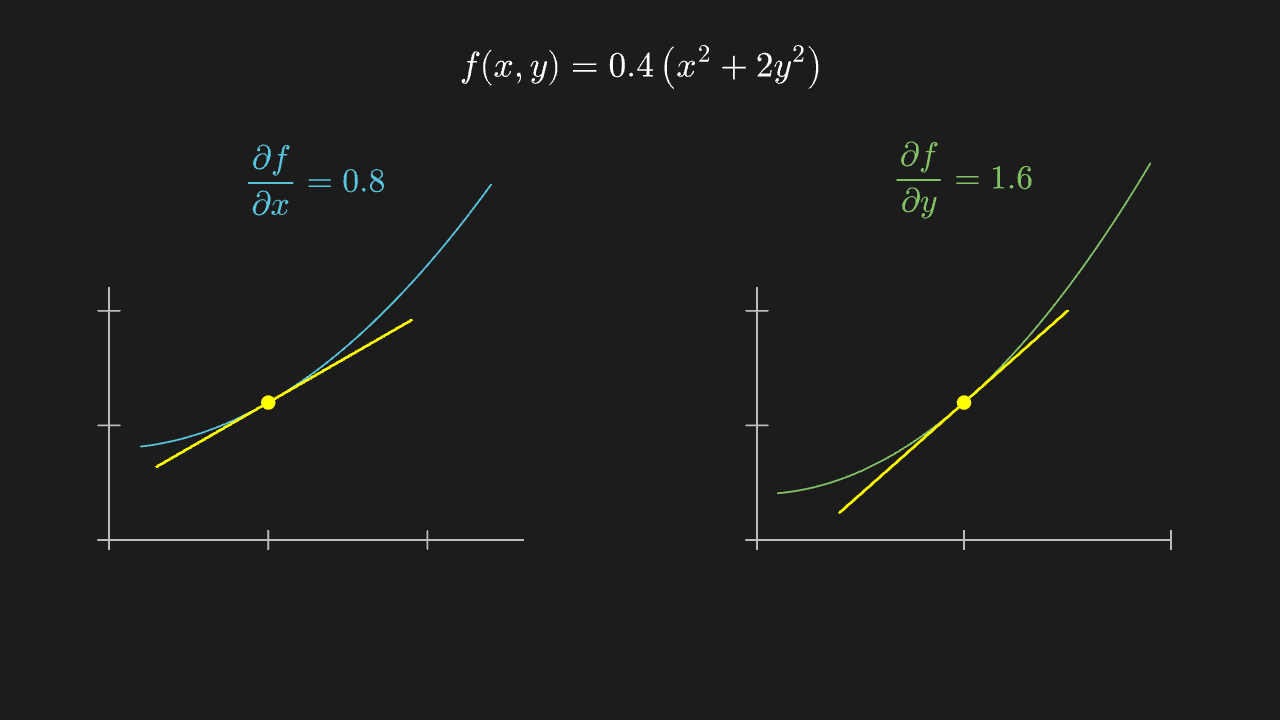
"""偏导数：分别固定 y 与固定 x 去看的斜率

@expect 左边那块画的是「固定 y=1 时 f 随 x 的变化」，右边是「固定 x=1 时 f 随 y 的变化」，
        两块各有一条过切点 (1, 1.2) 的黄色切线，斜率分别是 0.8 与 1.6，右边明显更陡。
@note 讲解要点：多元函数的「导数」得先说要沿哪个方向走——固定另一个变量，就退回一元情形。
    图上 f(x,y)=0.4(x²+2y²) 在点 (1,1)：f_x=0.8x=0.8、f_y=1.6y=1.6，所以右边明显更陡。
"""

from manim import *


class PartialDerivativeScene(Scene):
    def construct(self):
        left = Axes(x_range=[0, 2.6, 1], y_range=[0, 2.2, 1], x_length=4.6, y_length=2.8,
                    tips=False, axis_config={"color": GRAY_B}).shift(LEFT * 3.6 + DOWN * 0.6)
        right = Axes(x_range=[0, 2.0, 1], y_range=[0, 2.2, 1], x_length=4.6, y_length=2.8,
                     tips=False, axis_config={"color": GRAY_B}).shift(RIGHT * 3.6 + DOWN * 0.6)

        # 固定 y0=1：g(x) = 0.4*(x^2 + 2) → 在 x0=1 处切点 (1, 1.2)、斜率 f_x = 0.8*1 = 0.8
        # 切线 y = 1.2 + 0.8(x-1)：x=0.3 → 0.64，x=1.9 → 1.92
        cut_x = left.plot(lambda x: 0.4 * (x ** 2 + 2), x_range=[0.2, 2.4], color=BLUE)
        tan_x = Line(left.c2p(0.3, 0.64), left.c2p(1.9, 1.92), color=YELLOW)
        dot_x = Dot(left.c2p(1, 1.2), color=YELLOW)

        # 固定 x0=1：h(y) = 0.4*(1 + 2y^2) → 在 y0=1 处切点 (1, 1.2)、斜率 f_y = 1.6*1 = 1.6
        # 切线 y = 1.2 + 1.6(y-1)：y=0.4 → 0.24，y=1.5 → 2.0
        cut_y = right.plot(lambda y: 0.4 * (1 + 2 * y ** 2), x_range=[0.1, 1.9], color=GREEN)
        tan_y = Line(right.c2p(0.4, 0.24), right.c2p(1.5, 2.0), color=YELLOW)
        dot_y = Dot(right.c2p(1, 1.2), color=YELLOW)

        labels = VGroup(
            MathTex(r"\frac{\partial f}{\partial x} = 0.8", color=BLUE, font_size=36).move_to([-3.6, 2.0, 0]),
            MathTex(r"\frac{\partial f}{\partial y} = 1.6", color=GREEN, font_size=36).move_to([3.6, 2.0, 0]),
            MathTex(r"f(x,y)=0.4\left(x^2+2y^2\right)", font_size=38).to_edge(UP),
        )

        self.play(Write(labels[2]), run_time=0.8)
        self.play(Create(left), Create(cut_x), Write(labels[0]), run_time=1.0)
        self.play(Create(right), Create(cut_y), Write(labels[1]), run_time=1.0)
        self.play(Create(tan_x), FadeIn(dot_x), run_time=0.7)
        self.play(Create(tan_y), FadeIn(dot_y), run_time=0.7)
        self.wait(0.4)

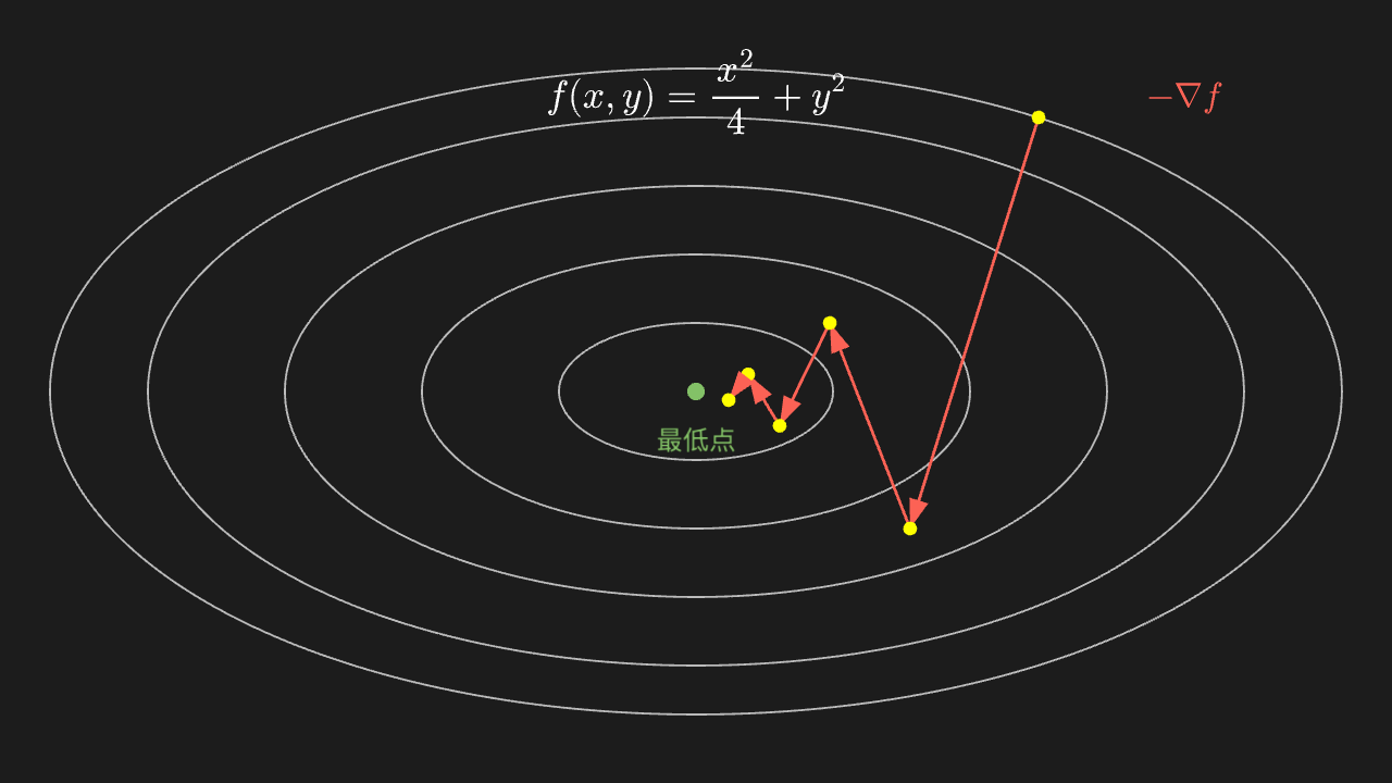
梯度下降：沿负梯度方向一步步走向最小值

五条同心椭圆是等高线（越里越低），折线从外圈锯齿状折向中心——步子沿负梯度在谷的两侧交替弹跳、一步步收窄，箭头标出每一步的方向。

画面

代码

"""梯度下降：沿负梯度方向一步步走向最小值

@expect 五条同心椭圆是等高线（越里越低），折线从外圈锯齿状折向中心——步子沿负梯度在谷的两侧交替弹跳、一步步收窄，箭头标出每一步的方向。
@note 讲解要点：等高线的法线方向就是梯度方向，所以「负梯度」总是垂直于当前等高线、指向更低的那一圈；
    步长 0.75 时 y 方向过冲（1-2·0.75<0），路径在谷两侧交替弹跳着收敛——「越到谷底走得越慢」的由来是梯度变小。
"""

from manim import *
import numpy as np


class GradientDescentScene(Scene):
    def construct(self):
        # f(x,y) = x^2/4 + y^2 的等高线：椭圆 x^2/4 + y^2 = r^2
        levels = VGroup(*[
            ParametricFunction(
                lambda t, r=r: [2 * r * np.cos(t), r * np.sin(t), 0],
                t_range=[0, TAU, 0.02],
                color=GRAY_B,
            )
            for r in [0.7, 1.4, 2.1, 2.8, 3.3]
        ])

        # 真实梯度下降：x ← x(1-α/2)、y ← y(1-2α)，α=0.75 时 y 过冲翻号，路径呈锯齿
        path_points = [
            [3.5, 2.8, 0],
            [3.5 * 0.625, 2.8 * -0.5, 0],
            [3.5 * 0.625**2, 2.8 * 0.25, 0],
            [3.5 * 0.625**3, 2.8 * -0.125, 0],
            [3.5 * 0.625**4, 2.8 * 0.0625, 0],
            [3.5 * 0.625**5, 2.8 * -0.03125, 0],
        ]
        dots = VGroup(*[Dot(point, radius=0.07, color=YELLOW) for point in path_points])
        arrows = VGroup(*[
            Arrow(path_points[index], path_points[index + 1], buff=0.12, color=RED, stroke_width=3)
            for index in range(len(path_points) - 1)
        ])
        center = Dot(ORIGIN, radius=0.09, color=GREEN)

        title = MathTex(r"f(x,y)=\frac{x^2}{4}+y^2", font_size=38).to_edge(UP)
        direction = MathTex(r"-\nabla f", color=RED, font_size=34).move_to([5.0, 3.0, 0])
        bottom_note = Text("最低点", font_size=26, color=GREEN).next_to(center, DOWN, buff=0.25)

        self.play(Create(levels), Write(title), run_time=1.0)
        self.play(FadeIn(center), Write(bottom_note), run_time=0.6)
        self.play(FadeIn(dots[0]), run_time=0.4)
        # dots[1:] 这种切片在适配层取不到子物体（下标才行），所以按下标走
        for index in range(len(arrows)):
            self.play(Create(arrows[index]), FadeIn(dots[index + 1]), run_time=0.6)
        self.play(Write(direction), run_time=0.5)
        self.wait(0.4)

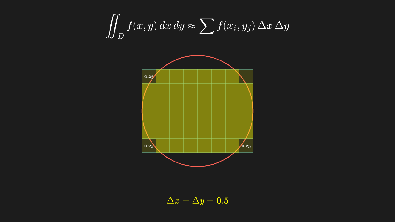
二重积分：把区域切成小方块

矩形区域内铺满小方格，落在圆内的格子被高亮，边上的格子只算一部分。

画面

代码

"""二重积分：把区域切成小方块

@expect 矩形区域内铺满小方格，落在圆内的格子被高亮，边上的格子只算一部分。
@note 讲解要点：二重积分就是「把区域切成很多小块、每块按 f 加权求和」的极限；格子越细越准。
    高亮用的是「格心在圆内」这一判据——这正是数值积分里最常用的采样方式。
"""

from manim import *
import numpy as np


class DoubleIntegralGridScene(Scene):
    def construct(self):
        dx, dy = 0.5, 0.5
        xs = np.arange(-2.0, 2.0, dx)
        ys = np.arange(-1.5, 1.5, dy)

        inside = VGroup()
        partial = VGroup()
        outside = VGroup()
        partial_cells = []
        for x0 in xs:
            for y0 in ys:
                cell = Rectangle(width=dx, height=dy, stroke_width=1)
                cell.move_to([float(x0) + dx / 2, float(y0) + dy / 2, 0])
                cx, cy = float(x0) + dx / 2, float(y0) + dy / 2
                r2 = cx ** 2 + cy ** 2
                if r2 <= 4.0:
                    cell.set_fill(YELLOW, 0.45)
                    inside.add(cell)
                else:
                    # 格心在外但方块与圆相交：四角至少一角落圆内，按角点比例估权重
                    corners = [(cx - dx / 2, cy - dy / 2), (cx + dx / 2, cy - dy / 2),
                               (cx - dx / 2, cy + dy / 2), (cx + dx / 2, cy + dy / 2)]
                    frac = sum(1.0 for ux, uy in corners if ux ** 2 + uy ** 2 <= 4.0) / 4.0
                    if frac > 0:
                        cell.set_fill(YELLOW, 0.15)
                        partial.add(cell)
                        partial_cells.append((cx, cy, frac))
                    else:
                        outside.add(cell)

        circle = Circle(radius=2.0, color=RED, stroke_width=3)
        weight_marks = VGroup()
        for cx, cy, frac in partial_cells[:3]:
            mark = Text(f"{frac:.2f}", font_size=16, color=WHITE)
            mark.move_to([cx, cy, 0])
            weight_marks.add(mark)
        labels = VGroup(
            MathTex(r"\iint_D f(x,y)\,dx\,dy \approx \sum f(x_i,y_j)\,\Delta x\,\Delta y", font_size=38).to_edge(UP),
            MathTex(r"\Delta x = \Delta y = 0.5", color=YELLOW, font_size=32).to_edge(DOWN, buff=0.6),
        )

        self.play(Write(labels[0]), run_time=0.8)
        self.play(Create(outside), Create(circle), run_time=1.0)
        self.play(LaggedStart(*[FadeIn(cell) for cell in inside], lag_ratio=0.02), run_time=1.6)
        self.play(FadeIn(partial), Write(weight_marks), run_time=0.8)
        self.play(Write(labels[1]), run_time=0.5)
        self.wait(0.4)

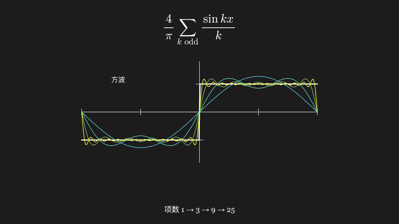
傅里叶级数逼近方波

一条方波（台阶状）与四条部分和曲线叠在一起：项数越多，平坦段越平、跳变处越陡，但跳变点附近始终有一个小过冲（吉布斯现象）。

画面

代码

"""傅里叶级数逼近方波

@expect 一条方波（台阶状）与四条部分和曲线叠在一起：项数越多，平坦段越平、跳变处越陡，
        但跳变点附近始终有一个小过冲（吉布斯现象）。
@note 讲解要点：用正弦波叠出方波，需要无穷多项；有限项一定会「振铃」。
    部分和由 numpy 直接算好再交给 plot_line_graph——比在 lambda 里逐点求和快得多，也更稳。
"""

from manim import *
import numpy as np


class FourierSquareScene(Scene):
    def construct(self):
        ax = Axes(
            x_range=[-PI, PI, PI / 2],
            y_range=[-1.8, 1.8, 1],
            x_length=8.4,
            y_length=3.6,
            tips=False,
            axis_config={"color": GRAY_B},
        )
        xs = np.linspace(-np.pi, np.pi, 240)
        square = np.sign(np.sin(xs))
        square[square == 0] = 1.0

        square_graph = ax.plot_line_graph(xs, square, add_vertex_dots=False,
                                          line_color=WHITE, stroke_width=4)
        square_label = Text("方波", font_size=24, color=WHITE).move_to([-2.9, 1.15, 0])
        partials = VGroup()
        for terms, color in [(1, BLUE), (3, TEAL), (9, GREEN), (25, YELLOW)]:
            ys = np.zeros_like(xs)
            for k in range(1, terms + 1, 2):
                ys += (4 / np.pi) * np.sin(k * xs) / k
            partials.add(ax.plot_line_graph(xs, ys, add_vertex_dots=False, line_color=color))

        note = Text("项数 1 → 3 → 9 → 25", font_size=26, color=WHITE).to_edge(DOWN, buff=0.35)
        title = MathTex(r"\frac{4}{\pi}\sum_{k\ \text{odd}}\frac{\sin kx}{k}", font_size=42).to_edge(UP)

        self.play(Create(ax), Create(square_graph), Write(square_label), run_time=1.0)
        self.play(Write(title), run_time=0.8)
        for curve in partials:
            self.play(Create(curve), run_time=0.8)
        self.play(Write(note), run_time=0.5)
        self.wait(0.5)

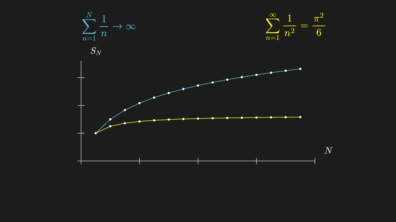
部分和：调和级数发散 vs Σ1/n² 收敛

蓝线（调和级数部分和）一路上爬、看不到头；黄线（1/n² 部分和）很快压平并停住。

画面

代码

"""部分和：调和级数发散 vs Σ1/n² 收敛

@expect 蓝线（调和级数部分和）一路上爬、看不到头；黄线（1/n² 部分和）很快压平并停住。
@note 讲解要点：通项都趋于 0，但一个收敛一个发散——「通项趋于 0」只是必要条件。
    两条都用 plot_line_graph 画在 n 上，横轴就是项数。
"""

from manim import *
import numpy as np


class SeriesPartialSumScene(Scene):
    def construct(self):
        ax = Axes(
            x_range=[0, 16, 4],
            y_range=[0, 3.6, 1],
            x_length=8.4,
            y_length=3.6,
            tips=False,
            axis_config={"color": GRAY_B},
        )
        ns = np.arange(1, 16)
        harmonic = np.cumsum(1.0 / ns)
        quadratic = np.cumsum(1.0 / ns ** 2)

        harmonic_graph = ax.plot_line_graph(ns, harmonic, add_vertex_dots=True,
                                            line_color=BLUE, vertex_dot_radius=0.04)
        quadratic_graph = ax.plot_line_graph(ns, quadratic, add_vertex_dots=True,
                                            line_color=YELLOW, vertex_dot_radius=0.04)

        labels = VGroup(
            MathTex(r"\sum_{n=1}^{N}\frac{1}{n} \to \infty", color=BLUE, font_size=36).move_to([-3.2, 3.05, 0]),
            MathTex(r"\sum_{n=1}^{\infty}\frac{1}{n^2} = \frac{\pi^2}{6}", color=YELLOW, font_size=36).move_to([3.5, 3.05, 0]),
        )
        axis_labels = ax.get_axis_labels(x_label="N", y_label="S_N")

        self.play(Create(ax), Write(axis_labels), run_time=1.0)
        self.play(Write(labels[1]), Create(quadratic_graph), run_time=1.2)
        self.play(Write(labels[0]), Create(harmonic_graph), run_time=1.5)
        self.wait(0.4)