线性代数
矩阵乘向量、行列式面积、奇异矩阵、投影、Gram–Schmidt、特征分解、秩与零空间、基变换、最小二乘、二次型与 SVD。
本页 12 条示例。代码引自 corpus/examples/math-linear/,截图为真机渲染的终态。
矩阵乘向量 = 列的线性组合
两个列向量 a₁ / a₂(蓝、绿)按系数各自伸缩后拼成平行四边形,对角线就是 A·x。
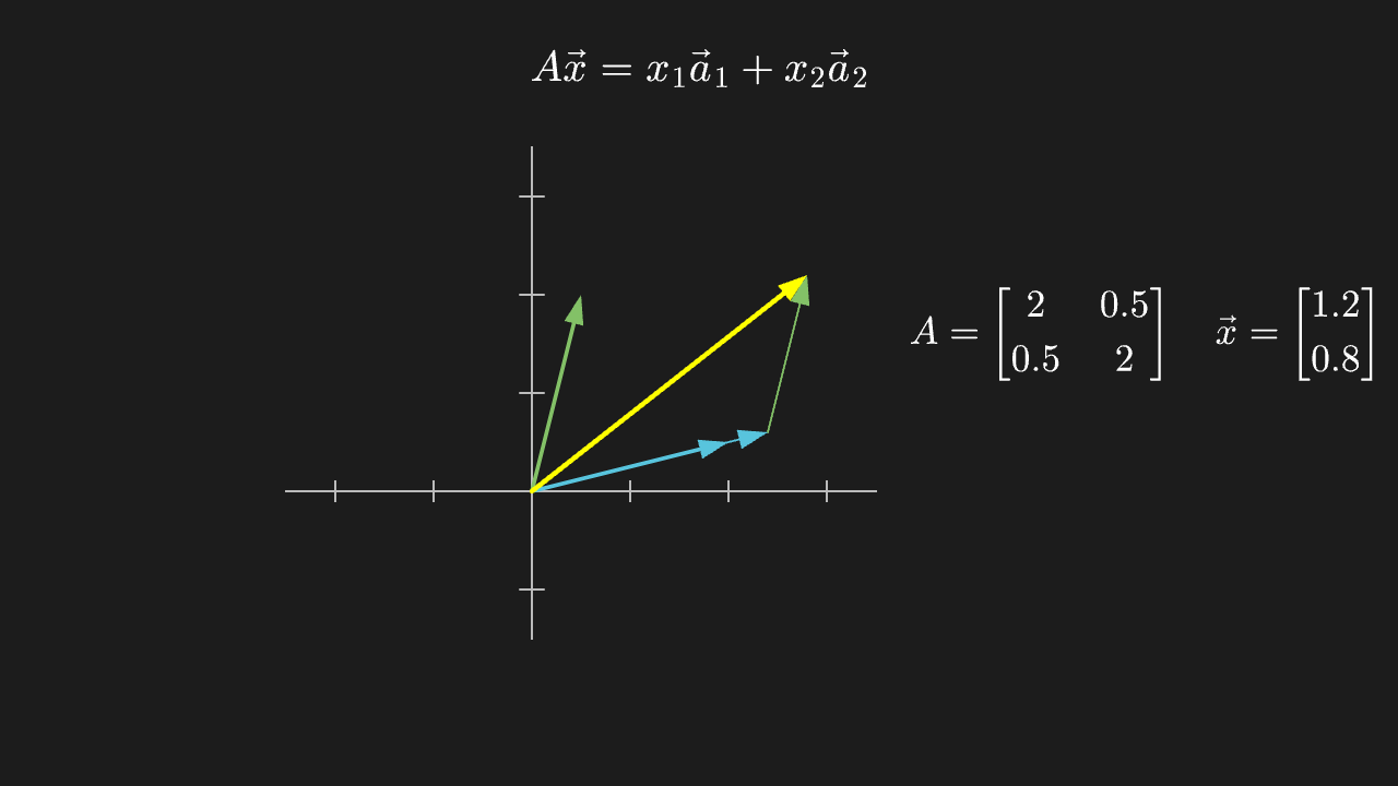
"""矩阵乘向量 = 列的线性组合

@expect 两个列向量 a₁ / a₂(蓝、绿)按系数各自伸缩后拼成平行四边形,对角线就是 A·x。
@note 讲解要点:A·x 不是「一堆乘法」,而是**用 x 的分量去加权 A 的各列再相加**——
    所以矩阵的列就是「基向量被搬到哪儿去了」,这句话是理解线性变换的入口。
"""

from manim import *


class MatrixVectorProductScene(Scene):
    def construct(self):
        # 等比:x 与 y 每个单位都用同一长度,否则正交/平行看起来会歪
        ax = Axes(
            x_range=[-2.5, 3.5, 1],
            y_range=[-1.5, 3.5, 1],
            x_length=6.0,
            y_length=5.0,
            tips=False,
            axis_config={"color": GRAY_B},
        ).shift(LEFT * 1.2)

        a1 = Arrow(ax.c2p(0, 0), ax.c2p(2, 0.5), buff=0, color=BLUE, stroke_width=4)
        a2 = Arrow(ax.c2p(0, 0), ax.c2p(0.5, 2), buff=0, color=GREEN, stroke_width=4)
        # x = (1.2, 0.8):结果 = 1.2*a1 + 0.8*a2
        x1, x2 = 1.2, 0.8
        scaled1 = Arrow(ax.c2p(0, 0), ax.c2p(2 * x1, 0.5 * x1), buff=0, color=BLUE, stroke_width=2)
        scaled2 = Arrow(ax.c2p(2 * x1, 0.5 * x1), ax.c2p(2 * x1 + 0.5 * x2, 0.5 * x1 + 2 * x2),
                        buff=0, color=GREEN, stroke_width=2)
        result = Arrow(ax.c2p(0, 0), ax.c2p(2 * x1 + 0.5 * x2, 0.5 * x1 + 2 * x2),
                       buff=0, color=YELLOW, stroke_width=5)
        # 平行四边形的另一条边(虚线补全)
        ghost = DashedLine(ax.c2p(0, 0), ax.c2p(0.5 * x2, 2 * x2), color=GREEN)

        formula = MathTex(r"A\vec x = x_1\vec a_1 + x_2\vec a_2", font_size=42).to_edge(UP)
        matrix = MathTex(r"A=\begin{bmatrix} 2 & 0.5 \\ 0.5 & 2 \end{bmatrix}",
                         r"\quad \vec x=\begin{bmatrix} 1.2 \\ 0.8 \end{bmatrix}", font_size=38).move_to([4.5, 0.6, 0])

        self.play(Create(ax), Write(formula), run_time=1.0)
        self.play(GrowArrow(a1), GrowArrow(a2), run_time=0.8)
        self.play(Write(matrix), run_time=0.6)
        self.play(GrowArrow(scaled1), GrowArrow(scaled2), run_time=1.0)
        self.play(Create(ghost), run_time=0.4)
        self.play(GrowArrow(result), run_time=0.8)
        self.play(Indicate(result, color=YELLOW), run_time=0.6)
        self.wait(0.4)
行列式的几何意义:单位正方形的面积被放大 |det| 倍
网格里那个黄色单位正方形被拉成平行四边形,面积从 1 变成 2(det=2)。
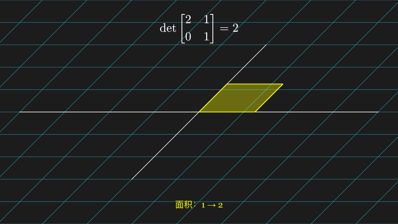
"""行列式的几何意义:单位正方形的面积被放大 |det| 倍

@expect 网格里那个黄色单位正方形被拉成平行四边形,面积从 1 变成 2(det=2)。
@note 讲解要点:行列式不是「算出来的一堆乘积」,它是**面积(体积)的缩放因子**;
    为负表示翻转了朝向,为 0 表示整个平面被压扁(下一页那条)。
"""

from manim import *


class DeterminantAreaScene(Scene):
    def construct(self):
        plane = NumberPlane(
            x_range=[-4, 4, 1],
            y_range=[-3, 3, 1],
            x_length=6.4,
            y_length=4.8,
            background_line_style={"stroke_color": GRAY_D, "stroke_width": 1},
        )
        unit = Square(side_length=1, color=YELLOW, stroke_width=3).set_fill(YELLOW, 0.35)
        unit.move_to([0.5, 0.5, 0])
        det_label = MathTex(r"\det\begin{bmatrix} 2 & 1 \\ 0 & 1 \end{bmatrix} = 2", font_size=42).to_edge(UP)
        area_label = Text("面积:1 → 2", font_size=30, color=YELLOW).to_edge(DOWN, buff=0.5)

        self.play(Create(plane), run_time=1.0)
        self.play(FadeIn(unit), Write(det_label), run_time=0.8)
        self.play(ApplyMatrix([[2, 1], [0, 1]], VGroup(plane, unit)), run_time=2.0)
        self.play(Write(area_label), run_time=0.6)
        self.wait(0.4)
奇异矩阵:det=0 把整个平面压成一条线
网格连同黄色方块被压扁成一条斜线,方块永远变不回有面积的形状。
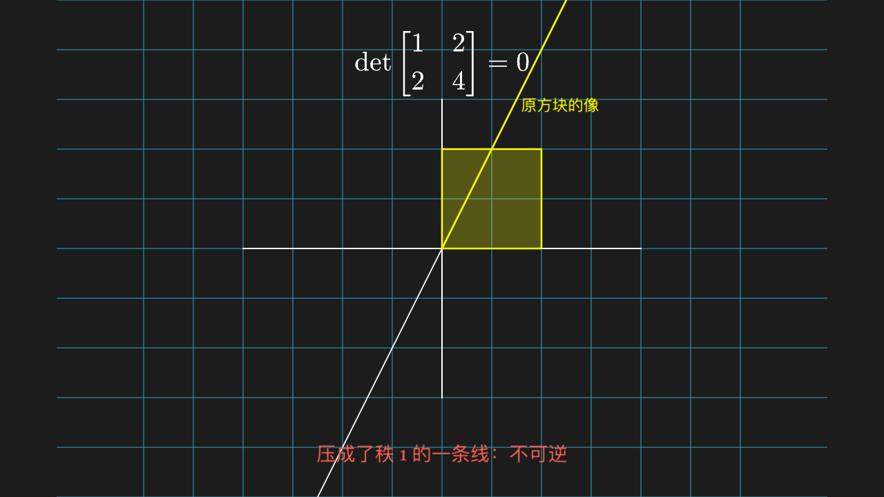
"""奇异矩阵:det=0 把整个平面压成一条线

@expect 网格连同黄色方块被压扁成一条斜线,方块永远变不回有面积的形状。
@note 讲解要点:det=0 ⇔ 矩阵不可逆 ⇔ 信息丢了(不同的点被映到同一个点),
    所以「逆矩阵不存在」不是代数上的刁难,而是几何上「压扁了就展不平」。
"""

from manim import *


class SingularMatrixScene(Scene):
    def construct(self):
        plane = NumberPlane(
            x_range=[-4, 4, 1],
            y_range=[-3, 3, 1],
            x_length=6.4,
            y_length=4.8,
            background_line_style={"stroke_color": GRAY_D, "stroke_width": 1},
        )
        block = Square(side_length=1.6, color=YELLOW, stroke_width=3).set_fill(YELLOW, 0.35)
        block.move_to([0.8, 0.8, 0])
        det_label = MathTex(r"\det\begin{bmatrix} 1 & 2 \\ 2 & 4 \end{bmatrix} = 0", font_size=42).to_edge(UP)
        note = Text("压成了秩 1 的一条线:不可逆", font_size=30, color=RED).to_edge(DOWN, buff=0.5)

        # 变换前留低透明度 ghost 在原位,ApplyMatrix 只作用实体组
        ghost_plane = plane.copy().set_opacity(0.25)
        ghost_block = block.copy().set_opacity(0.25)
        image_label = Text("原方块的像", font_size=24, color=YELLOW).move_to([1.9, 2.3, 0])

        self.play(Create(plane), run_time=1.0)
        self.play(FadeIn(block), Write(det_label), run_time=0.8)
        self.play(FadeIn(ghost_plane), FadeIn(ghost_block), run_time=0.6)
        self.play(ApplyMatrix([[1, 2], [2, 4]], VGroup(plane, block)), run_time=2.0)
        self.play(Write(note), FadeIn(image_label), run_time=0.6)
        self.wait(0.4)
正交投影:b 在 a 上的影子
从 b 的末端落一条虚线垂直打到 a 直线上,交点处有个直角符号;黄色箭头就是投影向量。
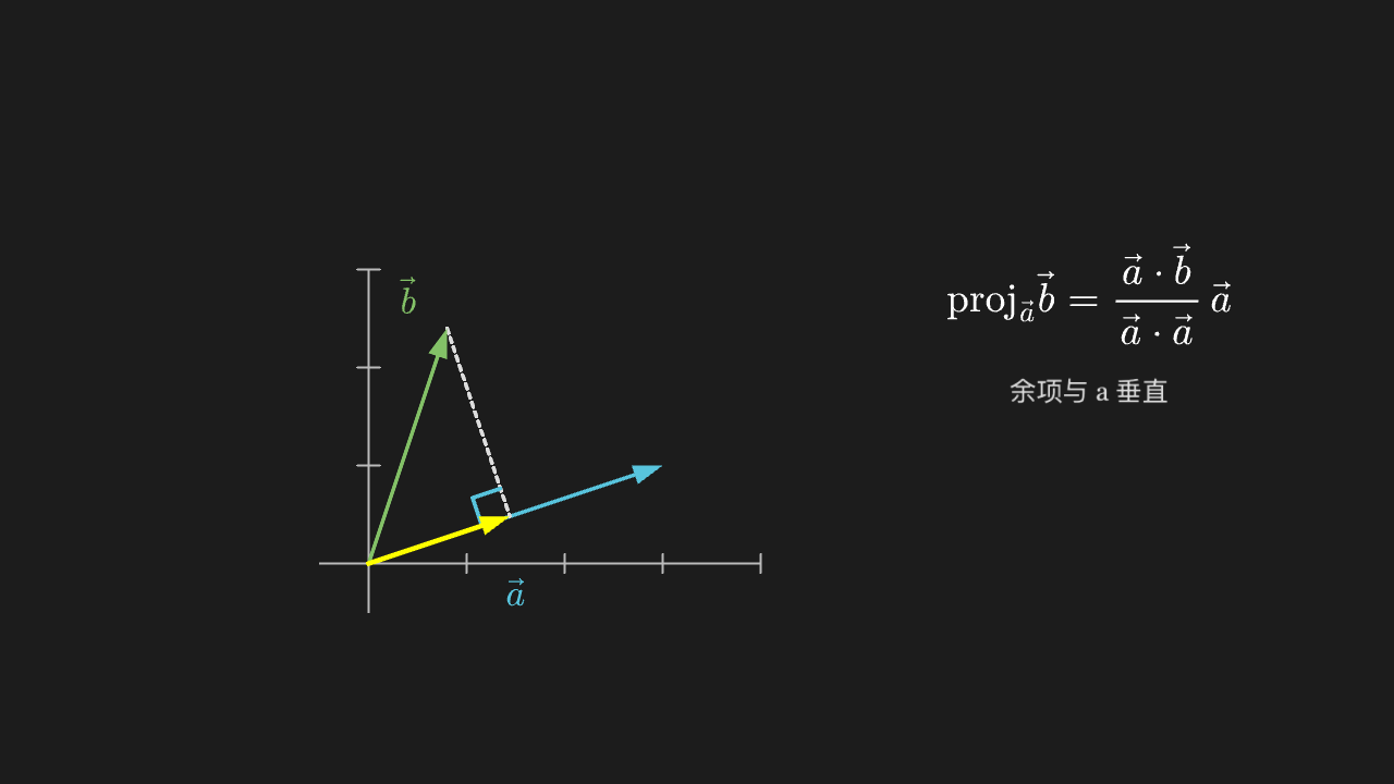
"""正交投影:b 在 a 上的影子

@expect 从 b 的末端落一条虚线垂直打到 a 直线上,交点处有个直角符号;黄色箭头就是投影向量。
@note 讲解要点:投影 = 「沿 a 方向能解释多少 b,剩下的部分与 a 垂直」。
    直角符号是关键——投影的余项一定垂直于 a,最小二乘、正交基都从这条性质长出来。
"""

from manim import *


class OrthogonalProjectionScene(Scene):
    def construct(self):
        ax = Axes(
            x_range=[-0.5, 4, 1],
            y_range=[-0.5, 3, 1],
            x_length=4.5,
            y_length=3.5,
            tips=False,
            axis_config={"color": GRAY_B},
        ).shift(LEFT * 1.6 + DOWN * 0.5)

        a_end = ax.c2p(3, 1)
        b_end = ax.c2p(0.8, 2.4)
        # proj = (a·b/|a|²) a = 0.48 a = (1.44, 0.48)
        proj_end = ax.c2p(1.44, 0.48)

        vec_a = Arrow(ax.c2p(0, 0), a_end, buff=0, color=BLUE, stroke_width=4)
        vec_b = Arrow(ax.c2p(0, 0), b_end, buff=0, color=GREEN, stroke_width=4)
        vec_p = Arrow(ax.c2p(0, 0), proj_end, buff=0, color=YELLOW, stroke_width=5)
        drop = DashedLine(b_end, proj_end, color=GRAY_A)
        mark = RightAngle(Line(ax.c2p(0, 0), proj_end), Line(proj_end, b_end), length=0.22)

        label_a = MathTex(r"\vec a", color=BLUE, font_size=36).next_to(vec_a, DOWN, buff=0.15)
        label_b = MathTex(r"\vec b", color=GREEN, font_size=36).next_to(vec_b, UP, buff=0.15)
        formula = MathTex(
            r"\mathrm{proj}_{\vec a}\vec b = \frac{\vec a\cdot\vec b}{\vec a\cdot\vec a}\,\vec a",
            font_size=40,
        ).move_to([4.0, 1.0, 0])
        note = Text("余项与 a 垂直", font_size=26, color=GRAY_A).move_to([4.0, 0.0, 0])

        self.play(Create(ax), run_time=0.8)
        self.play(GrowArrow(vec_a), GrowArrow(vec_b), Write(label_a), Write(label_b), run_time=1.0)
        self.play(Write(formula), run_time=0.8)
        self.play(Create(drop), Create(mark), run_time=0.7)
        self.play(GrowArrow(vec_p), run_time=0.8)
        self.play(Write(note), run_time=0.5)
        self.wait(0.4)
Gram–Schmidt:把第二个向量减掉它在第一个上的投影
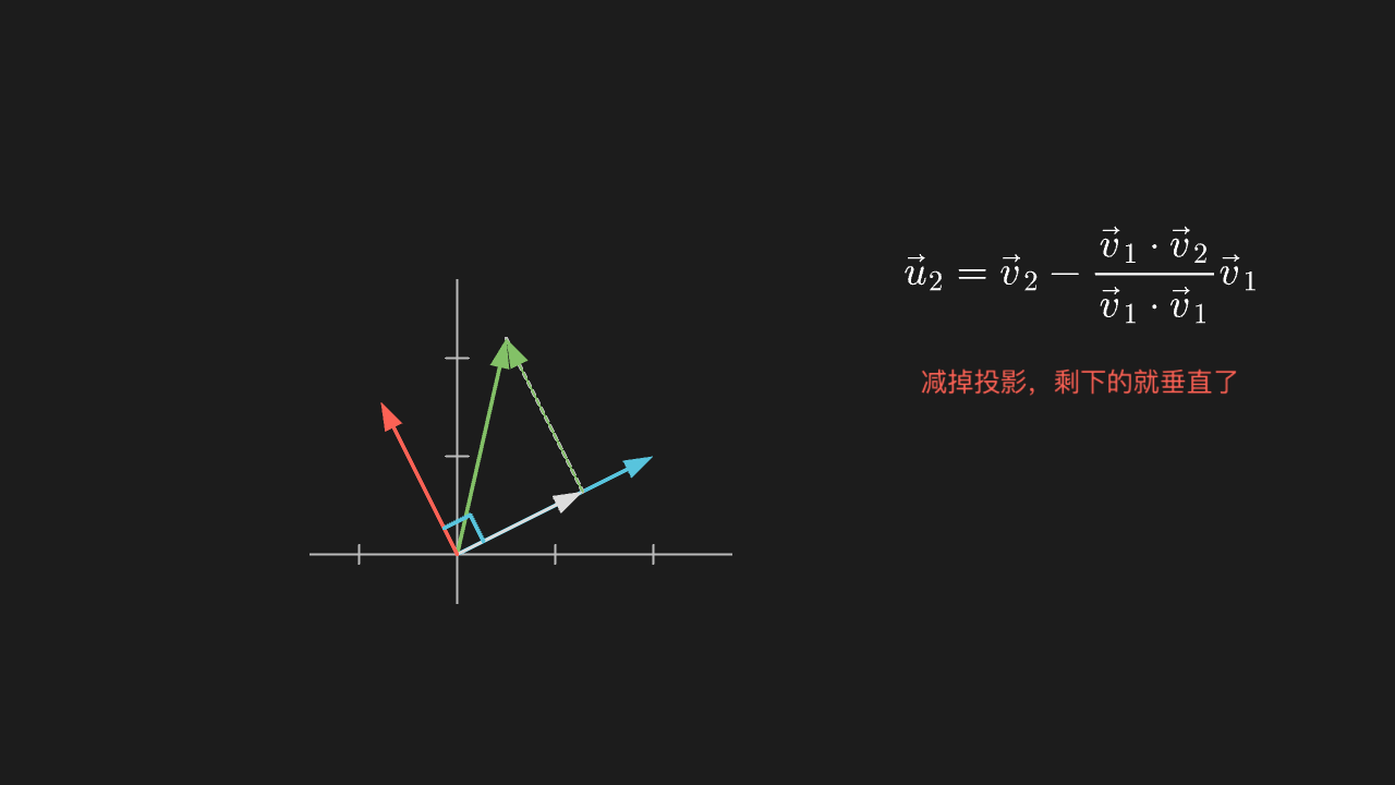
绿色向量沿虚线滑到红色位置后,与蓝色向量成直角(交点处有直角符号)。
"""Gram–Schmidt:把第二个向量减掉它在第一个上的投影

@expect 绿色向量沿虚线滑到红色位置后,与蓝色向量成直角(交点处有直角符号)。
@note 讲解要点:正交化的动作只有一句「减掉投影」——余下的部分自动垂直于前者。
    这就是 QR 分解、正交基、乃至傅里叶系数一路复用的同一个动作。
"""

from manim import *


class GramSchmidtScene(Scene):
    def construct(self):
        ax = Axes(
            x_range=[-1.5, 2.8, 1],
            y_range=[-0.5, 2.8, 1],
            x_length=4.3,
            y_length=3.3,
            tips=False,
            axis_config={"color": GRAY_B},
        ).shift(LEFT * 1.8 + DOWN * 0.5)

        origin = ax.c2p(0, 0)
        v1_end = ax.c2p(2, 1)
        v2_end = ax.c2p(0.5, 2.2)
        # 投影 (a·b/a·a)a:a·b = 1 + 2.2 = 3.2,a·a = 5 → 0.64·(2,1) = (1.28, 0.64)
        proj_end = ax.c2p(1.28, 0.64)
        ortho_end = ax.c2p(0.5 - 1.28, 2.2 - 0.64)  # (-0.78, 1.56)

        v1 = Arrow(origin, v1_end, buff=0, color=BLUE, stroke_width=4)
        v2 = Arrow(origin, v2_end, buff=0, color=GREEN, stroke_width=4)
        proj = Arrow(origin, proj_end, buff=0, color=GRAY_A, stroke_width=3)
        ortho = Arrow(origin, ortho_end, buff=0, color=RED, stroke_width=4)
        slide = Arrow(ax.c2p(1.28, 0.64), ax.c2p(0.5 - 1.28 + 1.28, 2.2 - 0.64 + 0.64 - 0.0),
                      buff=0, color=GREEN, stroke_width=2)
        drop = DashedLine(v2_end, ax.c2p(1.28, 0.64), color=GRAY_B)
        mark = RightAngle(Line(origin, v1_end), Line(origin, ortho_end), length=0.2)

        formula = MathTex(r"\vec u_2 = \vec v_2 - \frac{\vec v_1\cdot\vec v_2}{\vec v_1\cdot\vec v_1}\vec v_1",
                          font_size=40).move_to([3.9, 1.2, 0])
        note = Text("减掉投影,剩下的就垂直了", font_size=26, color=RED).move_to([3.9, 0.1, 0])

        self.play(Create(ax), run_time=0.8)
        self.play(GrowArrow(v1), GrowArrow(v2), run_time=0.8)
        self.play(Create(drop), GrowArrow(proj), run_time=0.7)
        self.play(Write(formula), run_time=0.8)
        self.play(Create(slide), run_time=0.5)
        self.play(GrowArrow(ortho), Create(mark), run_time=0.9)
        self.play(Write(note), run_time=0.5)
        self.wait(0.4)
特征方向:变换后方向不变的向量
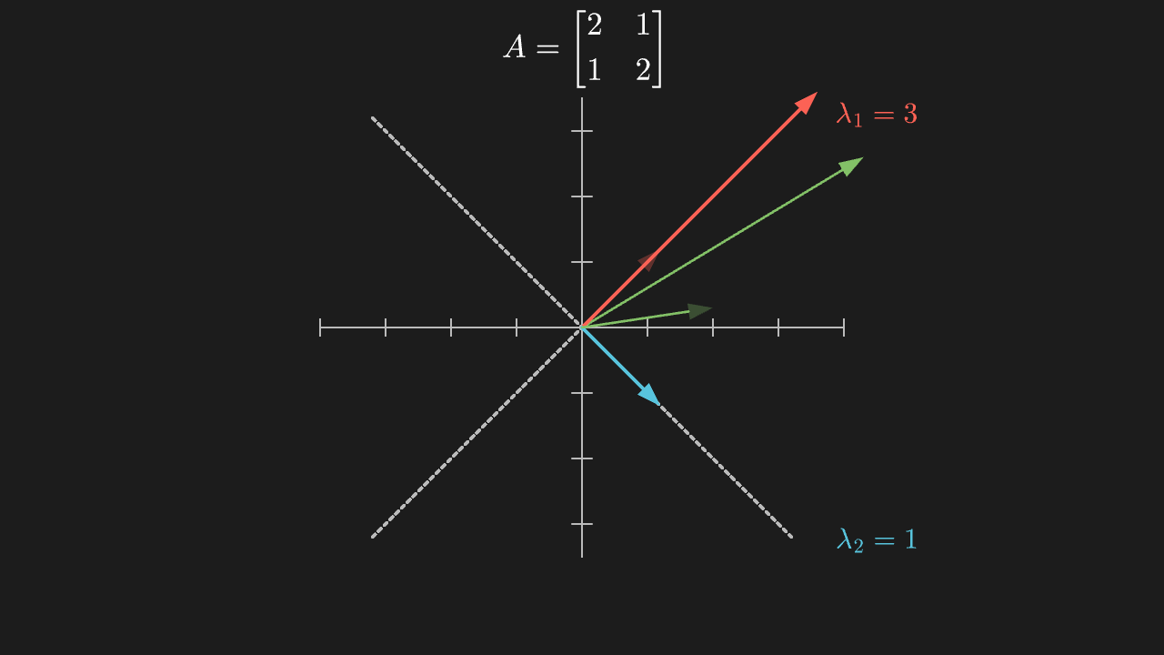
两条虚线标出的方向上,向量变换后仍落在同一条直线上(只被拉长/压短);第三个向量明显偏转。变换前三根向量以半透明 ghost 留在画面,与变换后的实色向量形成 before/after 对照。
"""特征方向:变换后方向不变的向量

@expect 两条虚线标出的方向上,向量变换后仍落在同一条直线上(只被拉长/压短);第三个向量明显偏转。
    变换前三根向量以半透明 ghost 留在画面,与变换后的实色向量形成 before/after 对照。
@note 讲解要点:特征向量就是「这个变换自己的方向」——沿它走只改长度不改方向,长度比就是特征值。
    这里 (1,1) 被拉 3 倍、(1,-1) 保持 1 倍,所以 A 的两个特征值是 3 和 1。
"""

from manim import *


class EigenvectorScene(Scene):
    def construct(self):
        ax = Axes(
            x_range=[-4, 4, 1],
            y_range=[-3.5, 3.5, 1],
            x_length=6.4,
            y_length=5.6,
            tips=False,
            axis_config={"color": GRAY_B},
        )

        # 两条特征方向上的参考直线(虚)
        line_1 = DashedLine(ax.c2p(-3.2, -3.2), ax.c2p(3.2, 3.2), color=GRAY_B)
        line_2 = DashedLine(ax.c2p(-3.2, 3.2), ax.c2p(3.2, -3.2), color=GRAY_B)

        v1 = Arrow(ax.c2p(0, 0), ax.c2p(1.2, 1.2), buff=0, color=RED, stroke_width=4)
        v2 = Arrow(ax.c2p(0, 0), ax.c2p(1.2, -1.2), buff=0, color=BLUE, stroke_width=4)
        v3 = Arrow(ax.c2p(0, 0), ax.c2p(2.0, 0.3), buff=0, color=GREEN, stroke_width=3)

        label_1 = MathTex(r"\lambda_1 = 3", color=RED, font_size=34).move_to([3.6, 2.6, 0])
        label_2 = MathTex(r"\lambda_2 = 1", color=BLUE, font_size=34).move_to([3.6, -2.6, 0])
        matrix = MathTex(r"A=\begin{bmatrix} 2 & 1 \\ 1 & 2 \end{bmatrix}", font_size=38).move_to([0, 3.4, 0])

        self.play(Create(ax), Create(line_1), Create(line_2), run_time=1.0)
        self.play(GrowArrow(v1), GrowArrow(v2), GrowArrow(v3), Write(matrix), run_time=1.0)

        # 变换前 ghost:半透明副本留在画面,不参与变换,供 before/after 对照
        ghosts = [m.copy().set_opacity(0.3) for m in (v1, v2, v3)]
        self.play(*[FadeIn(g, scale=0.9) for g in ghosts], run_time=0.6)

        # 变换只作用在原向量上:箭头不进 ApplyMatrix,按手算端点重画后 Transform
        A = [[2, 1], [1, 2]]

        def apply_A(x, y):
            return (A[0][0] * x + A[0][1] * y, A[1][0] * x + A[1][1] * y)

        ends = [(1.2, 1.2), (1.2, -1.2), (2.0, 0.3)]
        colors_widths = [(RED, 4), (BLUE, 4), (GREEN, 3)]
        new_arrows = [
            Arrow(ax.c2p(0, 0), ax.c2p(*apply_A(x, y)), buff=0, color=c, stroke_width=w)
            for (x, y), (c, w) in zip(ends, colors_widths)
        ]
        self.play(
            Transform(v1, new_arrows[0]),
            Transform(v2, new_arrows[1]),
            Transform(v3, new_arrows[2]),
            run_time=2.0,
        )
        self.play(Write(label_1), Write(label_2), run_time=0.7)
        self.play(Circumscribe(v3, color=GREEN), run_time=0.6)
        self.wait(0.4)
零空间:被映到 0 的那些方向
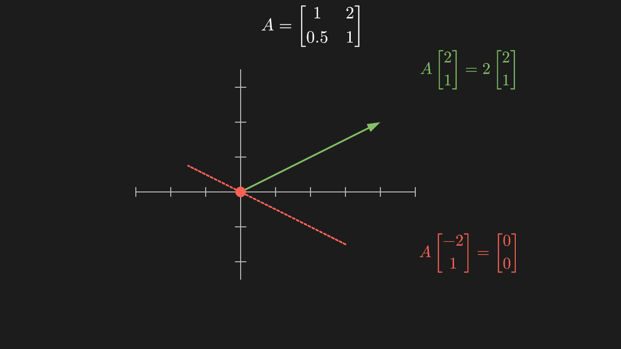
沿 (-2,1) 方向的箭头(红)变换后缩成一个点(原点处红点);另一个方向(绿)变换后变成它的 2 倍长。
"""零空间:被映到 0 的那些方向

@expect 沿 (-2,1) 方向的箭头(红)变换后缩成一个点(原点处红点);另一个方向(绿)变换后变成它的 2 倍长。
@note 讲解要点:零空间不是「什么都没有」,而是「本来在这里、被矩阵丢掉的整个方向」。
    秩数 = 留下来(有像)的维数,二者互为一对:留下来 1 维,被丢掉就 1 维。
"""

from manim import *


class RankNullspaceScene(Scene):
    def construct(self):
        ax = Axes(
            x_range=[-3, 5, 1],
            y_range=[-2.5, 3.5, 1],
            x_length=6.4,
            y_length=4.8,
            tips=False,
            axis_config={"color": GRAY_B},
        ).shift(LEFT * 0.8)

        null_line = DashedLine(ax.c2p(3, -1.5), ax.c2p(-1.5, 0.75), color=RED)
        null_vec = Arrow(ax.c2p(0, 0), ax.c2p(-2, 1), buff=0, color=RED, stroke_width=4)
        live_vec = Arrow(ax.c2p(0, 0), ax.c2p(2, 1), buff=0, color=GREEN, stroke_width=4)
        zero_dot = Dot(ax.c2p(0, 0), radius=0.12, color=RED)

        matrix = MathTex(r"A=\begin{bmatrix} 1 & 2 \\ 0.5 & 1 \end{bmatrix}", font_size=38).move_to([0, 3.4, 0])
        to_zero = MathTex(r"A\begin{bmatrix}-2\\1\end{bmatrix}=\begin{bmatrix}0\\0\end{bmatrix}",
                          color=RED, font_size=36).move_to([3.6, -1.8, 0])
        kept = MathTex(r"A\begin{bmatrix}2\\1\end{bmatrix}=2\begin{bmatrix}2\\1\end{bmatrix}",
                       color=GREEN, font_size=36).move_to([3.6, 2.4, 0])

        self.play(Create(ax), run_time=0.8)
        self.play(GrowArrow(null_vec), GrowArrow(live_vec), Write(matrix), run_time=1.0)
        self.play(Write(kept), run_time=0.6)
        # 箭头不进 ApplyMatrix:A·(-2,1)=(0,0) 缩成原点红点;A·(2,1)=(4,2) 变 2 倍长
        live_new = Arrow(ax.c2p(0, 0), ax.c2p(4, 2), buff=0, color=GREEN, stroke_width=4)
        self.play(ReplacementTransform(null_vec, zero_dot),
                  Transform(live_vec, live_new), run_time=2.0)
        self.play(Create(null_line), Write(to_zero), run_time=0.8)
        self.play(Circumscribe(live_vec, color=GREEN), run_time=0.6)
        self.wait(0.4)
基变换:同一个向量的两套坐标
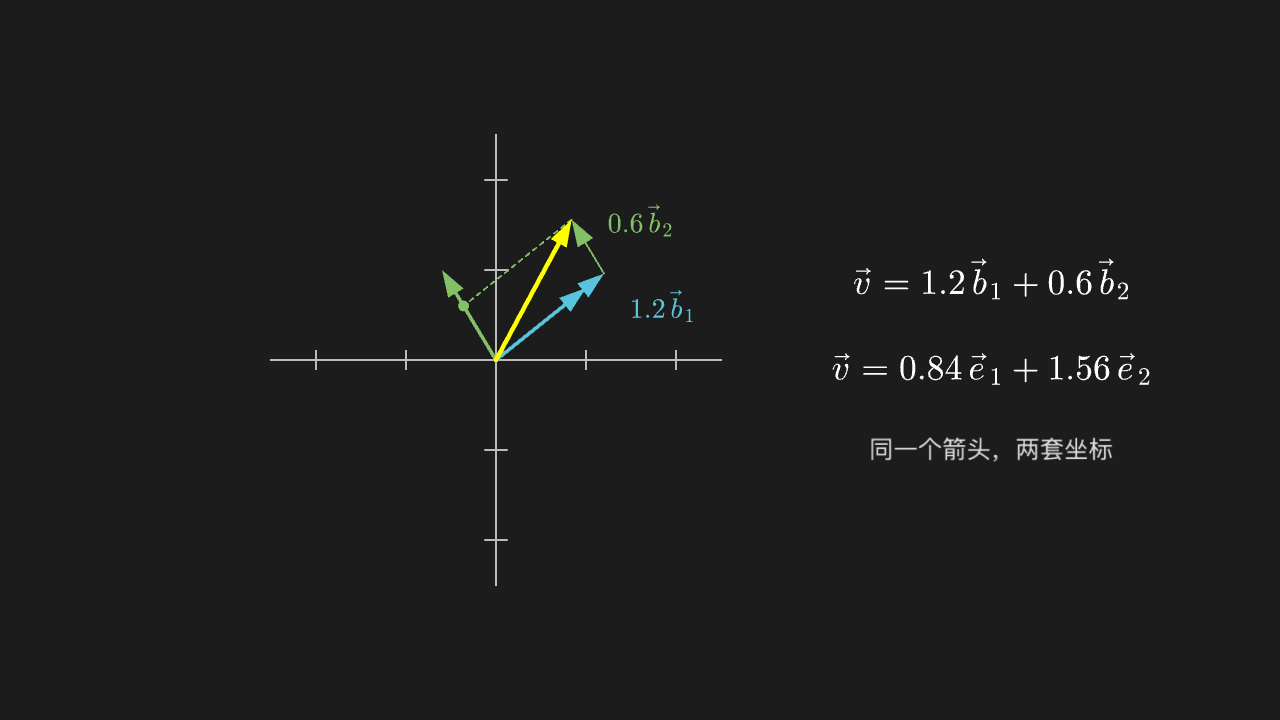
蓝色基与绿色基合成一个平行四边形(0.6·b₂ 那条闭合边用绿色虚线补全,并标注 1.2·b₁ / 0.6·b₂),黄色向量沿它们走的方式就是 (1.2, 0.6);换成标准基去看,同一根箭头的坐标变成另一组数。
"""基变换:同一个向量的两套坐标

@expect 蓝色基与绿色基合成一个平行四边形(0.6·b₂ 那条闭合边用绿色虚线补全,并标注 1.2·b₁ / 0.6·b₂),
        黄色向量沿它们走的方式就是 (1.2, 0.6);换成标准基去看,同一根箭头的坐标变成另一组数。
@note 讲解要点:向量本身没变,变的是「用哪两把尺子量」。所以「坐标」永远是相对基而言的,
    这句话一懂,相似矩阵 A = P⁻¹BP 就不再神秘。
"""

from manim import *


class BasisChangeScene(Scene):
    def construct(self):
        ax = Axes(
            x_range=[-2.5, 2.5, 1],
            y_range=[-2.5, 2.5, 1],
            x_length=5.0,
            y_length=5.0,
            tips=False,
            axis_config={"color": GRAY_B},
        ).shift(LEFT * 1.6)

        b1 = Arrow(ax.c2p(0, 0), ax.c2p(1, 0.8), buff=0, color=BLUE, stroke_width=4)
        b2 = Arrow(ax.c2p(0, 0), ax.c2p(-0.6, 1), buff=0, color=GREEN, stroke_width=4)
        # v = 1.2*b1 + 0.6*b2 = (1.2 - 0.36, 0.96 + 0.6) = (0.84, 1.56)
        step1 = Arrow(ax.c2p(0, 0), ax.c2p(1.2, 0.96), buff=0, color=BLUE, stroke_width=2)
        step2 = Arrow(ax.c2p(1.2, 0.96), ax.c2p(0.84, 1.56), buff=0, color=GREEN, stroke_width=2)
        # 平行四边形的闭合边(v 端点 → 0.6·b₂ 角点,平行于 b₁):虚线 ghost 补全
        closing = DashedLine(ax.c2p(0.84, 1.56), ax.c2p(-0.36, 0.6), color=GREEN, stroke_width=2)
        corner = Dot(ax.c2p(-0.36, 0.6), radius=0.06, color=GREEN)
        vec = Arrow(ax.c2p(0, 0), ax.c2p(0.84, 1.56), buff=0, color=YELLOW, stroke_width=5)
        # 重合的 1.2·b₁ 与粗蓝 b₁ 用标注区分
        label_step1 = MathTex(r"1.2\,\vec b_1", color=BLUE, font_size=30).move_to(ax.c2p(1.85, 0.6))
        label_step2 = MathTex(r"0.6\,\vec b_2", color=GREEN, font_size=30).move_to(ax.c2p(1.6, 1.55))

        coords_new = MathTex(r"\vec v = 1.2\,\vec b_1 + 0.6\,\vec b_2", font_size=38).move_to([3.9, 0.9, 0])
        coords_std = MathTex(r"\vec v = 0.84\,\vec e_1 + 1.56\,\vec e_2", font_size=38).move_to([3.9, -0.1, 0])
        note = Text("同一个箭头,两套坐标", font_size=26, color=GRAY_A).move_to([3.9, -1.0, 0])

        self.play(Create(ax), run_time=0.8)
        self.play(GrowArrow(b1), GrowArrow(b2), run_time=0.8)
        self.play(Write(coords_new), run_time=0.6)
        self.play(GrowArrow(step1), GrowArrow(step2), Create(closing), Create(corner), run_time=1.0)
        self.play(Write(label_step1), Write(label_step2), run_time=0.6)
        self.play(GrowArrow(vec), run_time=0.8)
        self.play(Write(coords_std), Write(note), run_time=0.8)
        self.wait(0.4)
旋转矩阵的复合:转两次 30° 等于转一次 60°
网格与黄色方块先被转 30°、再转 30°,两次之后的姿态与「一次转 60°」(虚线参考)完全重合。
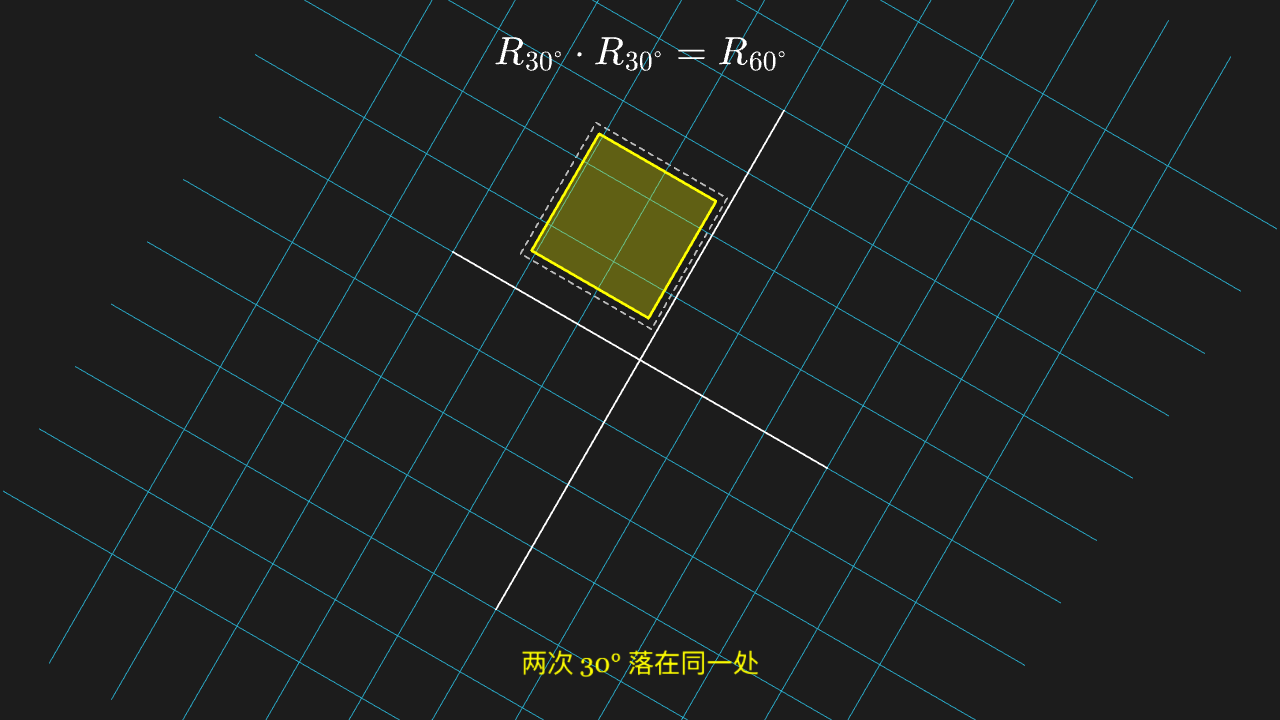
"""旋转矩阵的复合:转两次 30° 等于转一次 60°

@expect 网格与黄色方块先被转 30°、再转 30°,两次之后的姿态与「一次转 60°」(虚线参考)完全重合。
@note 讲解要点:矩阵乘法就是「先做右边那个、再做左边那个」,两个旋转矩阵乘起来还是旋转矩阵——
    这就是「矩阵乘法为什么这么定义」的动机。
"""

from manim import *
import math


class RotationCompositionScene(Scene):
    def construct(self):
        plane = NumberPlane(
            x_range=[-4, 4, 1],
            y_range=[-3, 3, 1],
            x_length=6.4,
            y_length=4.8,
            background_line_style={"stroke_color": GRAY_D, "stroke_width": 1},
        )
        block = Square(side_length=1.5, color=YELLOW, stroke_width=3).set_fill(YELLOW, 0.3)
        block.move_to([1.2, 0.9, 0])
        figure = VGroup(plane, block)

        half = math.pi / 6  # 30°
        r30 = [[math.cos(half), -math.sin(half)], [math.sin(half), math.cos(half)]]

        # 一次转 60° 的参考位置:虚线方块(手算角点)且外扩一圈,让「完全重合」可对照
        whole = math.pi / 3  # 60°
        target_center = [
            1.2 * math.cos(whole) - 0.9 * math.sin(whole),
            1.2 * math.sin(whole) + 0.9 * math.cos(whole),
            0,
        ]
        half_s = 0.75
        corners = []
        for sx in (-1, 1):
            for sy in (-1, 1):
                px, py = sx * half_s, sy * half_s
                corners.append([
                    target_center[0] + px * math.cos(whole) - py * math.sin(whole),
                    target_center[1] + px * math.sin(whole) + py * math.cos(whole),
                    0,
                ])
        ring = [0, 1, 3, 2]  # 角点环序
        target = VGroup(*[
            DashedLine(corners[ring[i]], corners[ring[(i + 1) % 4]], color=GRAY_B, stroke_width=2)
            for i in range(4)
        ]).scale(1.12)

        formula = MathTex(r"R_{30^\circ} \cdot R_{30^\circ} = R_{60^\circ}", font_size=42).move_to([0, 3.4, 0])
        note = Text("两次 30° 落在同一处", font_size=28, color=YELLOW).to_edge(DOWN, buff=0.45)

        self.play(Create(plane), FadeIn(target), Write(formula), run_time=1.0)
        self.play(FadeIn(block), run_time=0.4)
        self.play(ApplyMatrix(r30, VGroup(plane, block)), run_time=1.5)
        self.play(ApplyMatrix(r30, VGroup(plane, block)), run_time=1.5)
        self.play(Write(note), run_time=0.6)
        self.play(Flash(target, color=GRAY_A, line_length=0.25, flash_radius=1.2), run_time=0.8)
        self.wait(0.4)
最小二乘:拟合直线与残差
五个数据点上方有一条蓝色拟合直线,每个点到直线的竖直残差用灰色虚线画出、长短一目了然。
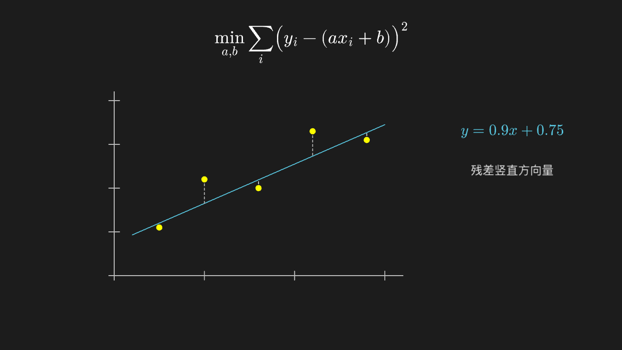
"""最小二乘:拟合直线与残差

@expect 五个数据点上方有一条蓝色拟合直线,每个点到直线的竖直残差用灰色虚线画出、长短一目了然。
@note 讲解要点:数据不可能刚好排在一条线上,所以「解不存在」;退一步求**让残差平方和最小**的那条线。
    残差竖线与直线垂直(图的纵横比一致),所以这套图里直角是看得出来的。
"""

from manim import *


class LeastSquaresScene(Scene):
    def construct(self):
        ax = Axes(
            x_range=[0, 3.2, 1],
            y_range=[0, 4.2, 1],
            x_length=6.6,
            y_length=4.2,
            tips=False,
            axis_config={"color": GRAY_B},
        ).shift(LEFT * 1.2 + DOWN * 0.2)

        xs = [0.5, 1.0, 1.6, 2.2, 2.8]
        ys = [1.1, 2.2, 2.0, 3.3, 3.1]
        points = VGroup(*[Dot(ax.c2p(x, y), radius=0.07, color=YELLOW) for x, y in zip(xs, ys)])

        fit = ax.plot(lambda x: 0.9 * x + 0.75, x_range=[0.2, 3.0], color=BLUE)
        residuals = VGroup(*[
            DashedLine(ax.c2p(x, y), ax.c2p(x, 0.9 * x + 0.75), color=GRAY_B, stroke_width=2)
            for x, y in zip(xs, ys)
        ])

        title = MathTex(r"\min_{a,b}\sum_i\bigl(y_i - (ax_i+b)\bigr)^2", font_size=40).to_edge(UP)
        fit_label = MathTex(r"y = 0.9x + 0.75", color=BLUE, font_size=34).move_to([4.6, 1.0, 0])
        note = Text("残差竖直方向量", font_size=26, color=GRAY_A).move_to([4.6, 0.1, 0])

        self.play(Create(ax), Write(title), run_time=1.0)
        self.play(LaggedStart(*[FadeIn(dot) for dot in points], lag_ratio=0.15), run_time=1.0)
        self.play(Create(fit), Write(fit_label), run_time=0.9)
        self.play(LaggedStart(*[Create(line) for line in residuals], lag_ratio=0.12), run_time=1.0)
        self.play(Write(note), run_time=0.5)
        self.wait(0.4)
二次型:正定的椭圆 vs 不定的双曲
左边一组同心椭圆(正定:所有方向都往上弯),右边一对双曲分支(不定:有的方向往下弯)。
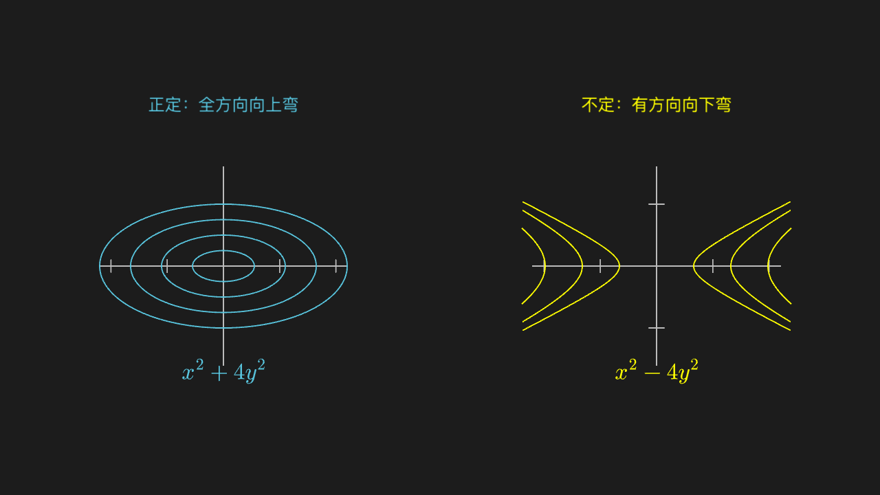
"""二次型:正定的椭圆 vs 不定的双曲

@expect 左边一组同心椭圆(正定:所有方向都往上弯),右边一对双曲分支(不定:有的方向往下弯)。
@note 讲解要点:二次型的「正定 / 不定」就是它的等高线是闭曲线还是开口曲线——
    判断正定不用背西尔维斯特判据,看形状就够了。
"""

from manim import *
import numpy as np


class QuadraticFormScene(Scene):
    def construct(self):
        left = Axes(
            x_range=[-2.2, 2.2, 1],
            y_range=[-1.6, 1.6, 1],
            x_length=4.0,
            y_length=3.2,
            tips=False,
            axis_config={"color": GRAY_B},
        ).shift(LEFT * 3.5 + DOWN * 0.3)
        right = Axes(
            x_range=[-2.2, 2.2, 1],
            y_range=[-1.6, 1.6, 1],
            x_length=4.0,
            y_length=3.2,
            tips=False,
            axis_config={"color": GRAY_B},
        ).shift(RIGHT * 3.5 + DOWN * 0.3)

        # 正定:x² + 4y² = r² 的等高线是椭圆
        ellipses = VGroup(*[
            ParametricFunction(lambda t, r=r: [r * np.cos(t), 0.5 * r * np.sin(t), 0],
                               t_range=[0, TAU, 0.02], color=BLUE).shift(LEFT * 3.5 + DOWN * 0.3)
            for r in [0.5, 1.0, 1.5, 2.0]
        ])
        # 不定:x² - 4y² = r² 的等高线是双曲分支(t_range 按每条 r 裁到轴框内,x 方向先出界)
        branches = VGroup()
        for r in [0.6, 1.2, 1.8]:
            t_max = min(np.arccosh(2.2 / r), np.arcsinh(1.6 / (0.5 * r))) - 0.02
            for sign in [1, -1]:
                branches.add(ParametricFunction(
                    lambda t, r=r, sign=sign, t_max=t_max: [sign * r * np.cosh(t), 0.5 * r * np.sinh(t), 0],
                    t_range=[-t_max, t_max, 0.02], color=YELLOW,
                ).shift(RIGHT * 3.5 + DOWN * 0.3))

        left_title = Text("正定:全方向向上弯", font_size=26, color=BLUE).move_to([-3.5, 2.3, 0])
        right_title = Text("不定:有方向向下弯", font_size=26, color=YELLOW).move_to([3.5, 2.3, 0])
        left_formula = MathTex(r"x^2+4y^2", color=BLUE, font_size=36).move_to([-3.5, -2.0, 0])
        right_formula = MathTex(r"x^2-4y^2", color=YELLOW, font_size=36).move_to([3.5, -2.0, 0])

        self.play(Create(left), Create(right), run_time=1.0)
        self.play(Write(left_title), Write(left_formula), run_time=0.6)
        self.play(LaggedStart(*[Create(item) for item in ellipses], lag_ratio=0.15), run_time=1.4)
        self.play(Write(right_title), Write(right_formula), run_time=0.6)
        self.play(LaggedStart(*[Create(item) for item in branches], lag_ratio=0.1), run_time=1.6)
        self.wait(0.4)
SVD 的几何含义:旋转 → 拉伸 → 再旋转
黄色圆经过三步(转 40°、沿轴拉伸、再转 -25°)变成一个倾斜的椭圆;中间那一步能明显看出两个方向被拉得不一样。
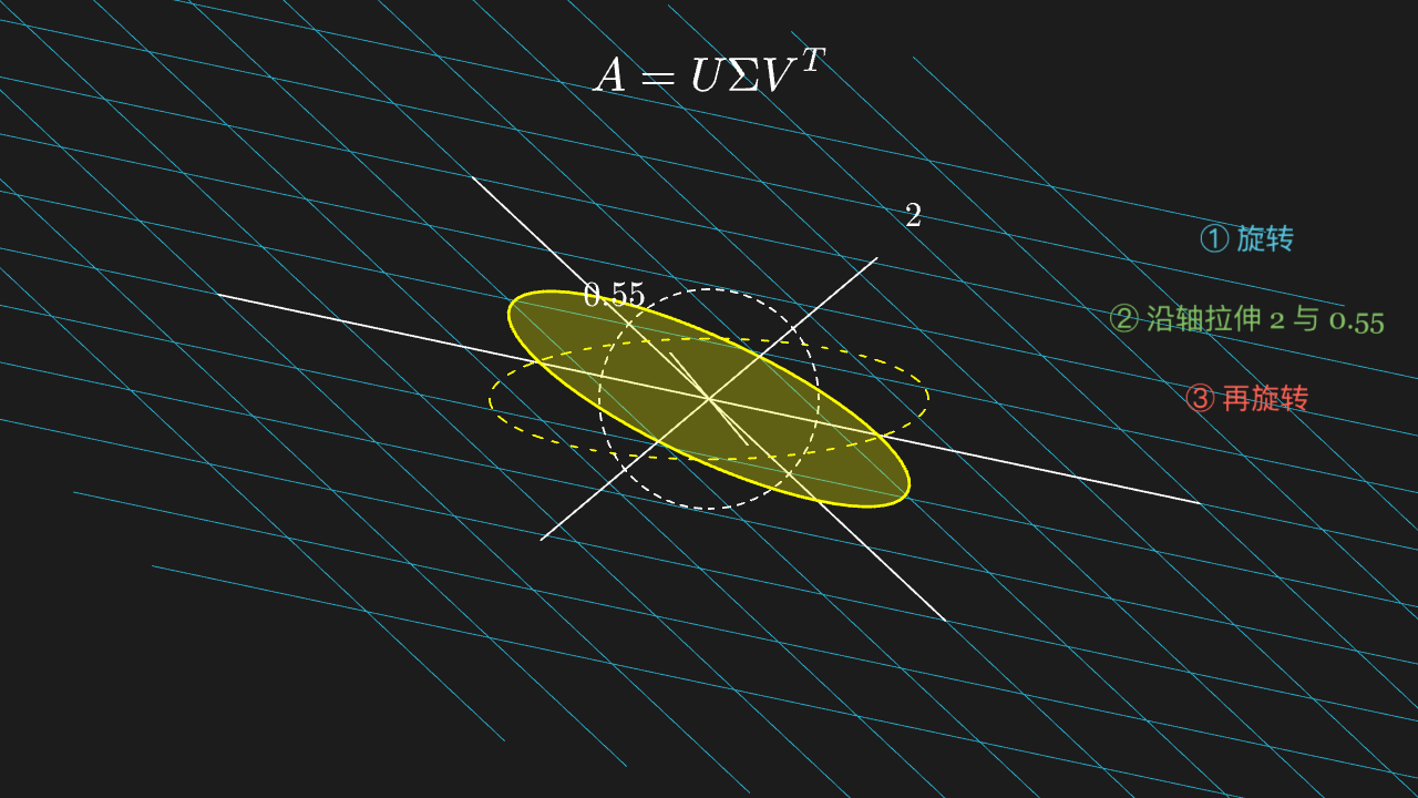
"""SVD 的几何含义:旋转 → 拉伸 → 再旋转

@expect 黄色圆经过三步(转 40°、沿轴拉伸、再转 -25°)变成一个倾斜的椭圆;
        中间那一步能明显看出两个方向被拉得不一样。
@note 讲解要点:任何矩阵都拆成「转一下、沿坐标轴拉一下、再转一下」——这就是 SVD。
    奇异值就是拉伸那两个倍数,左右两个旋转就是两套正交基的朝向。
"""

from manim import *
import math


class SvdGeometryScene(Scene):
    def construct(self):
        plane = NumberPlane(
            x_range=[-4, 4, 1],
            y_range=[-3, 3, 1],
            x_length=6.4,
            y_length=4.8,
            background_line_style={"stroke_color": GRAY_D, "stroke_width": 1},
        )
        disk = Circle(radius=1.1, color=YELLOW, stroke_width=3).set_fill(YELLOW, 0.3)
        figure = VGroup(plane, disk)

        theta1 = math.radians(40)
        v = [[math.cos(theta1), -math.sin(theta1)], [math.sin(theta1), math.cos(theta1)]]
        sigma = [[2.0, 0], [0, 0.55]]
        theta2 = math.radians(-25)
        u = [[math.cos(theta2), -math.sin(theta2)], [math.sin(theta2), math.cos(theta2)]]

        # \mathsf / \mathcal / \mathbb 一律别用:KaTeX 字体切换要动态加载,这里只会整段画成空
        caption = MathTex(r"A = U \Sigma V^{T}", font_size=46).move_to([0, 3.3, 0])
        # 混合说明逐行绝对定位在右侧留白区,不压图形
        step_1 = Text("① 旋转", font_size=28, color=BLUE).move_to([5.4, 1.6, 0])
        step_2 = Text("② 沿轴拉伸 2 与 0.55", font_size=28, color=GREEN).move_to([5.4, 0.8, 0])
        step_3 = Text("③ 再旋转", font_size=28, color=RED).move_to([5.4, 0.0, 0])

        # ghost 层:原始圆(白虚线)与中间态椭圆(黄虚线,主轴沿拉伸方向的 40° 朝向)
        ghost_circle = DashedVMobject(
            disk.copy().set_fill(opacity=0).set_stroke(WHITE, 2), num_dashes=48)
        ghost_mid = DashedVMobject(
            Ellipse(width=4.4, height=1.21, color=YELLOW, stroke_width=2)
            .set_fill(opacity=0)
            .rotate(theta1),
            num_dashes=48,
        )
        major_axis = Line(start=[-2.2 * math.cos(theta1), -2.2 * math.sin(theta1), 0],
                          end=[2.2 * math.cos(theta1), 2.2 * math.sin(theta1), 0],
                          stroke_color=WHITE, stroke_width=2)
        minor_axis = Line(start=[0.605 * math.cos(theta1 + math.pi / 2), 0.605 * math.sin(theta1 + math.pi / 2), 0],
                          end=[-0.605 * math.cos(theta1 + math.pi / 2), -0.605 * math.sin(theta1 + math.pi / 2), 0],
                          stroke_color=WHITE, stroke_width=2)
        # MathTex 定位一律 move_to 绝对坐标
        sigma_major = MathTex("2", font_size=34, color=WHITE).move_to([2.05, 1.85, 0])
        sigma_minor = MathTex("0.55", font_size=34, color=WHITE).move_to([-0.95, 1.05, 0])

        self.play(Create(plane), FadeIn(disk), Write(caption), run_time=1.0)
        self.play(Write(step_1), run_time=0.4)
        self.play(ApplyMatrix(v, figure), run_time=1.2)
        self.play(Write(step_2), run_time=0.4)
        self.play(ApplyMatrix(sigma, figure), run_time=1.2)
        self.play(FadeIn(ghost_mid), Write(step_3), run_time=0.6)
        self.play(ApplyMatrix(u, figure), run_time=1.2)
        self.play(FadeIn(ghost_circle), Create(major_axis), Create(minor_axis),
                  Write(sigma_major), Write(sigma_minor), run_time=0.8)
        self.wait(0.4)